26 Stats: Probability

Purpose: Probability is a quantitative measure of uncertainty. It is intimately tied to how we use distributions to model data and to how we express uncertainty. In order to do all these useful things, we’ll need to learn some basics about probability.

Reading: (None; this exercise is the reading.)

Topics: Frequency, probability, probability density function (PDF), cumulative distribution function (CDF)

“Probability is the most important concept in modern science, especially as nobody has the slightest notion what it means.” — Bertrand Russell

library(tidyverse)

## ── Attaching packages ─────────────────────────────────────── tidyverse 1.3.0 ──

## ✔ ggplot2 3.4.0      ✔ purrr   1.0.1 
## ✔ tibble  3.1.8      ✔ dplyr   1.0.10
## ✔ tidyr   1.2.1      ✔ stringr 1.5.0 
## ✔ readr   2.1.3      ✔ forcats 0.5.2

## ── Conflicts ────────────────────────────────────────── tidyverse_conflicts() ──
## ✖ dplyr::filter() masks stats::filter()
## ✖ dplyr::lag()    masks stats::lag()

26.1 Intuitive Definition

In the previous stats exercise, we learned about densities. In this exercise, we’re going to learn a more formal definition using probability. To introduce the idea of probability, let’s first think about frequency.

Imagine we have some set of events \(X\), and we’re considering some particular subset of cases that we’re interested in \(A\). For instance, imagine we’re rolling a 6-sided die, and we’re interested in cases when the number rolled is even. Then the subset of cases is \(A = \{2, 4, 6\}\), and an example run of rolls might be \(X = \{3, 5, 5, 2, 6, 1, 3, 3\}\).

The frequency with which events in \(A\) occurred for a run \(X\) is

\[F_X(A) \equiv \sum \frac{\text{Cases in set }A}{\text{Total Cases in }X}.\] For the example above, we have

\[\begin{aligned} A &= \{2, 4, 6\}, \\ X &= \{3, 5, 5, \mathbf{2}, \mathbf{6}, 1, 3, 3\}, \\ F_X(A) &= \frac{2}{8} = 1/4 \end{aligned}\]

Note that this definition of frequency considers both a set \(A\) and a sample \(X\). We need to define both \(A, X\) in order to compute a frequency.

As an example, let’s consider the set \(A\) to be the set of \(Z\) values such that \(-1.96 <= Z <= +1.96\): We denote this set as \(A = {Z | -1.96 <= Z <= +1.96}\). Let’s also let \(Z\) be a sample from a standard (mean = 0, sd = 1) normal. The following figure illustrates the set \(A\) against a standard normal density.

## NOTE: No need to change this!
tibble(z = seq(-3, +3, length.out = 500)) %>%
  mutate(d = dnorm(z)) %>%
  ggplot(aes(z, d)) +
  geom_ribbon(
    data = . %>% filter(-1.96 <= z, z <= +1.96),
    aes(ymin = 0, ymax = d, fill = "Set A"),
    alpha = 1 / 3
  ) +
  geom_line() +
  scale_fill_discrete(name = "")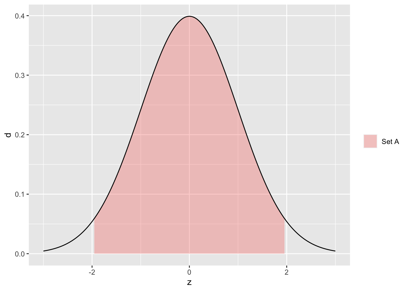

Note that a frequency is defined not in terms of a density, but rather in terms of a sample \(X\). The following example code draws a sample from a standard normal, and computes the frequency with which values in the sample \(X\) lie in the set \(A\).

## NOTE: No need to change this!
df_z <- tibble(z = rnorm(100))

df_z %>%
  mutate(in_A = (-1.96 <= z) & (z <= +1.96)) %>%
  summarize(count_total = n(), count_A = sum(in_A), fr = mean(in_A))

## # A tibble: 1 × 3
##   count_total count_A    fr
##         <int>   <int> <dbl>
## 1         100      98  0.98

Now it’s your turn!

26.1.1 q1 Let \(A = {Z | Z <= 0}\). Complete the following code to compute `count_total`, `count_A`, and `fr`. Before executing the code, make a prediction about the value of `fr`. Did the computed `fr` value match your prediction?

## NOTE: No need to change this!
df_z <- tibble(z = rnorm(100))

df_z %>%
  mutate(in_A = (z <= 0)) %>%
  summarize(count_total = n(), count_A = sum(in_A), fr = mean(in_A))

## # A tibble: 1 × 3
##   count_total count_A    fr
##         <int>   <int> <dbl>
## 1         100      52  0.52

Observations:

I predicted fr = 0.5
The value of fr I computed was 0.52, not quite the same. This is due to randomness in the calculation.

The following graph visualizes the set \(A = {z | z <= 0}\) against a standard normal density.

## NOTE: No need to change this!
tibble(z = seq(-3, +3, length.out = 500)) %>%
  mutate(d = dnorm(z)) %>%
  ggplot(aes(z, d)) +
  geom_ribbon(
    data = . %>% filter(z <= 0),
    aes(ymin = 0, ymax = d, fill = "Set A"),
    alpha = 1 / 3
  ) +
  geom_line() +
  scale_fill_discrete(name = "")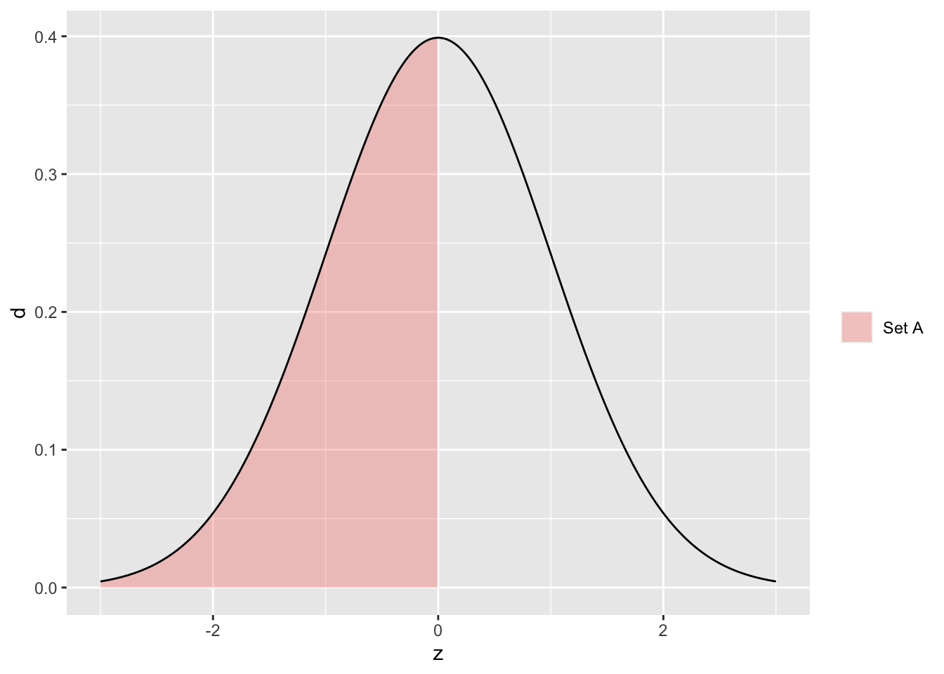

Based on this visual, we might expect fr = 0.5. This was (likely) not the value that our frequency took, but it is the precise value of the probability that \(Z <= 0.5\).

Remember in the previous stats exercise that when running rnorm with larger values of n we obtained histograms closer to the normal density? Something very similar happens with frequency and probability:

## NOTE: No need to change this!
map_dfr(
  c(10, 100, 1000, 1e4),
  function(n_samples) {
    tibble(
      z = rnorm(n = n_samples),
      n = n_samples
    ) %>%
      mutate(in_A = (z <= 0)) %>%
      summarize(count_total = n(), count_A = sum(in_A), fr = mean(in_A))
  }
)

## # A tibble: 4 × 3
##   count_total count_A    fr
##         <int>   <int> <dbl>
## 1          10       4 0.4  
## 2         100      39 0.39 
## 3        1000     510 0.51 
## 4       10000    4955 0.496

This is because probability is actually defined[1] in terms of the limit

\[\mathbb{P}_{\rho}[X \in A] = \lim_{n \to \infty} F_{X_n}(A),\]

where \(X_n\) is a sample of size \(n\) drawn from the density \(X_n \sim \rho\).[2]

26.1.2 q2: Modify the code below to consider the set \(A = {z | -1.96 <= z <= +1.96}\). What value does `fr` appear to be limiting towards?

## TASK: Modify the code below
map_dfr(
  c(10, 100, 1000, 1e4),
  function(n_samples) {
    tibble(
      z = rnorm(n = n_samples),
      n = n_samples
    ) %>%
      mutate(in_A = (-1.96 <= z) & (z <= +1.96)) %>%
      summarize(count_total = n(), count_A = sum(in_A), fr = mean(in_A))
  }
)

## # A tibble: 4 × 3
##   count_total count_A    fr
##         <int>   <int> <dbl>
## 1          10       9 0.9  
## 2         100      93 0.93 
## 3        1000     949 0.949
## 4       10000    9467 0.947

Observations:

fr is limiting towards ~0.95

Now that we know what probability is; let’s connect the idea to distributions.

26.2 Relation to Distributions

A continuous distribution models probability in terms of an integral

\[\mathbb{P}_{\rho}[X \in A] = \int_{-\infty}^{+\infty} \mathcal{I}_A(x)\rho(x)\,dx = \mathbb{E}_{\rho}[\mathcal{I}_A(X)]\]

where \(\mathcal{I}_A(x)\) is the indicator function; a function that takes the value \(1\) when \(x \in A\), and the value \(0\) when \(x \not\in A\). The \[\mathbb{E}[Y]\] denotes taking the mean of a random variable; this is also called the expectation of a random variable. The function \(\rho(x)\) is the density of the random variable—we’ll return to this idea in a bit.

This definition gives us a geometric way to think about probability; the distribution definition means probability is the area under the density curve within the set \(A\).

Before concluding this reading, let’s talk about two sticking points about distributions:

26.3 Sets vs Points

Note that for continuous distributions, the probability of a single point is zero. First, let’s gather some empirical evidence.

26.3.1 q3 Modify the code below to consider the set \(A = {z | z = 2}\).

Hint: Remember the difference between = and ==!

## TASK: Modify the code below
map_dfr(
  c(10, 100, 1000, 1e4),
  function(n_samples) {
    tibble(
      z = rnorm(n = n_samples),
      n = n_samples
    ) %>%
      mutate(in_A = (z == 2)) %>%
      summarize(count_total = n(), count_A = sum(in_A), fr = mean(in_A))
  }
)

## # A tibble: 4 × 3
##   count_total count_A    fr
##         <int>   <int> <dbl>
## 1          10       0     0
## 2         100       0     0
## 3        1000       0     0
## 4       10000       0     0

Observations:

fr is consistenly zero

We can also understand this phenomenon in terms of areas; the following graph visualizes the set \(A = {z | z = 2}\) against a standard normal.

## NOTE: No need to change this!
tibble(z = seq(-3, +3, length.out = 500)) %>%
  mutate(d = dnorm(z)) %>%
  ggplot(aes(z, d)) +
  geom_segment(
    data = tibble(z = 2, d = dnorm(2)),
    mapping = aes(z, 0, xend = 2, yend = d, color = "Set A")
  ) +
  geom_line() +
  scale_color_discrete(name = "")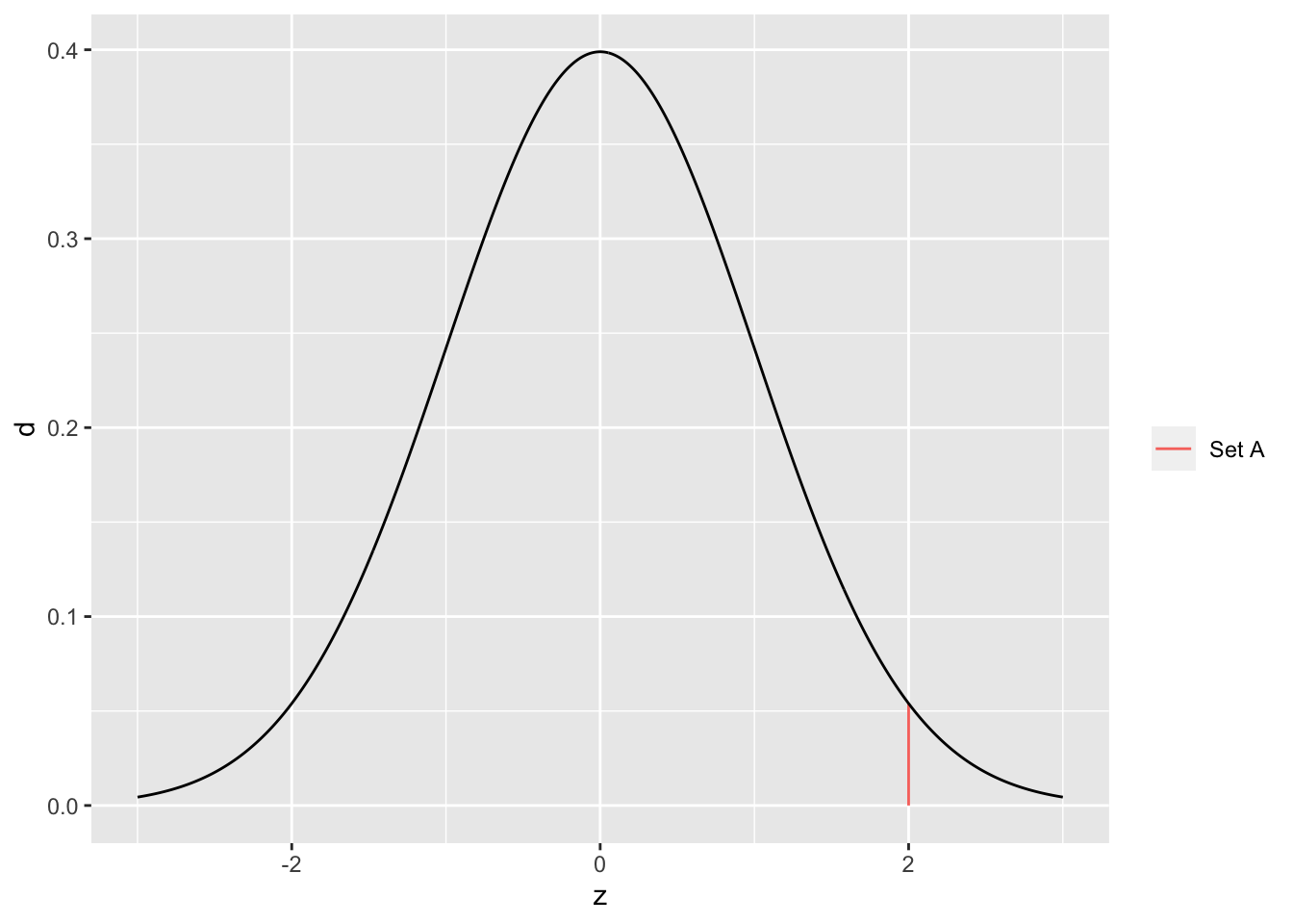

Note that this set \(A\) has nonzero height but zero width. Zero width corresponds to zero area, and thus zero probability.

This is weird. If we’re using a distribution to model something physical, say a material property, this means that any specific material property has zero probability of occurring. But in practice, some specific value will be realized! If you’d like to learn more, take a look at Note [3].

26.4 Two expressions of the same information

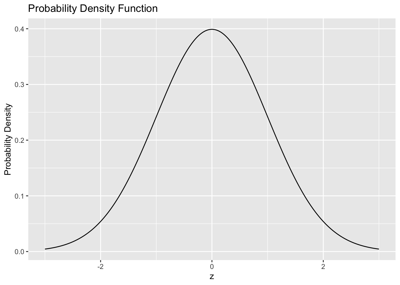
There is a bit more terminology associated with distributions. The \(\rho(x)\) we considered above is called a probability density function (PDF); it is the function we integrate in order to obtain a probability. In R, the PDF has the d prefix, for instance dnorm. For example, the standard normal has the following PDF.

tibble(z = seq(-3, +3, length.out = 1000)) %>%
  mutate(d = dnorm(z)) %>%

  ggplot(aes(z, d)) +
  geom_line() +
  labs(
    x = "z",
    y = "Probability Density",
    title = "Probability Density Function"
  )

There is also a cumulative distribution function, which is related to the PDF \(\rho(x)\) via

\[R(x) = \int_{-\infty}^x \rho(s) ds.\]

In R, the CDF has the prefix p, such as pnorm. For example, the standard normal has the following CDF.

tibble(z = seq(-3, +3, length.out = 1000)) %>%
  mutate(p = pnorm(z)) %>%

  ggplot(aes(z, p)) +
  geom_line() +
  labs(
    x = "z",
    y = "Probability",
    title = "Cumulative Distribution Function"
  )

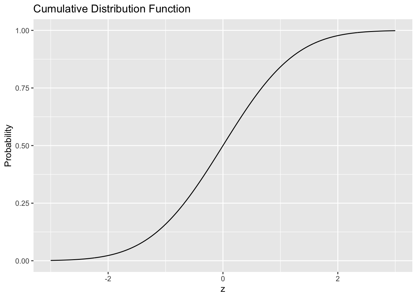
Note that, by definition, the CDF gives the probability over the set \(A(x) = {x' | x' <= x}\) (this is just all the values less than the value we’re considering \(x\)). Thus the CDF returns a probability (which explains the p prefix for R functions).

26.4.1 q4 Use `pnorm` to compute the probability that `Z ~ norm(mean = 0, sd = 1)` is less than or equal to zero. Compare this against your frequency prediction from q1.

## TASK: Compute the probability that Z <= 0, assign to p0
p0 <- pnorm(q = 0)
p0

## [1] 0.5

Use the following code to check your answer.

## NOTE: No need to change this
assertthat::assert_that(p0 == 0.5)

## [1] TRUE

print("Nice!")

## [1] "Nice!"

Observations:

I predicted fr = 0.5, which matches p0.

Note that when our set \(A\) is an interval, we can use the CDF to express the associated probability. Note that

\[\mathbb{P}_{\rho}[a <= X <= b] = \int_a^b \rho(x) dx = \int_{-\infty}^b \rho(x) dx - \int_{-\infty}^a \rho(x) dx.\]

26.4.2 q5 Using the identity above, use `pnorm` to compute the probability that \(-1.96 <= Z <= +1.96\) with `Z ~ norm(mean = 0, sd = 1)`.

## TASK: Compute the probability that -1.96 <= Z <= +1.96, assign to pI
pI <- pnorm(q = +1.96) - pnorm(q = -1.96)
pI

## [1] 0.9500042

Use the following code to check your answer.

## NOTE: No need to change this
assertthat::assert_that(abs(pI - 0.95) < 1e-3)

## [1] TRUE

print("Nice!")

## [1] "Nice!"

26.5 Notes

[1] This is where things get confusing and potentially controversial. This “limit of frequencies” definition of probability is called “Frequentist probability”, to distinguish it from a “Bayesian probability”. The distinction is meaningful but slippery. We won’t cover this distinction in this course. If you’re curious to learn more, my favorite video on Bayes vs Frequentist is by Kristin Lennox.

Note that even Bayesians use this Frequentist definition of probability, for instance in Markov Chain Monte Carlo, the workhorse of Bayesian computation.

[2] Technically these samples must be drawn independently and identically distributed, shortened to iid.

[3] 3Blue1Brown has a very nice video about continuous probabilities.

26 Stats: Probability

26.1 Intuitive Definition

26.1.1 q1 Let \(A = {Z | Z <= 0}\). Complete the following code to compute count_total, count_A, and fr. Before executing the code, make a prediction about the value of fr. Did the computed fr value match your prediction?

26.1.2 q2: Modify the code below to consider the set \(A = {z | -1.96 <= z <= +1.96}\). What value does fr appear to be limiting towards?

26.2 Relation to Distributions

26.3 Sets vs Points

26.3.1 q3 Modify the code below to consider the set \(A = {z | z = 2}\).

26.4 Two expressions of the same information

26.4.1 q4 Use pnorm to compute the probability that Z ~ norm(mean = 0, sd = 1) is less than or equal to zero. Compare this against your frequency prediction from q1.

26.4.2 q5 Using the identity above, use pnorm to compute the probability that \(-1.96 <= Z <= +1.96\) with Z ~ norm(mean = 0, sd = 1).

26.5 Notes

26.1.1 q1 Let \(A = {Z | Z <= 0}\). Complete the following code to compute `count_total`, `count_A`, and `fr`. Before executing the code, make a prediction about the value of `fr`. Did the computed `fr` value match your prediction?

26.1.2 q2: Modify the code below to consider the set \(A = {z | -1.96 <= z <= +1.96}\). What value does `fr` appear to be limiting towards?

26.4.1 q4 Use `pnorm` to compute the probability that `Z ~ norm(mean = 0, sd = 1)` is less than or equal to zero. Compare this against your frequency prediction from q1.

26.4.2 q5 Using the identity above, use `pnorm` to compute the probability that \(-1.96 <= Z <= +1.96\) with `Z ~ norm(mean = 0, sd = 1)`.