34 Data: Pipes and Placeholders
Purpose: The pipe %>% has additional functionality than what we’ve used so far. In this exercise we’ll learn about the placeholder ., which will give us more control over how data flows between our functions.
Reading: The Pipe
## ── Attaching core tidyverse packages ──────────────────────── tidyverse 2.0.0 ──
## ✔ dplyr     1.1.4     ✔ readr     2.1.5
## ✔ forcats   1.0.0     ✔ stringr   1.5.1
## ✔ ggplot2   3.5.2     ✔ tibble    3.2.1
## ✔ lubridate 1.9.4     ✔ tidyr     1.3.1
## ✔ purrr     1.0.4
## ── Conflicts ────────────────────────────────────────── tidyverse_conflicts() ──
## ✖ dplyr::filter() masks stats::filter()
## ✖ dplyr::lag()    masks stats::lag()
## ℹ Use the conflicted package (<http://conflicted.r-lib.org/>) to force all conflicts to become errors
34.0.1 q1 Re-write the following code to use the placeholder.
Hint: This may feel very simple, in which case good. This is not a trick question.
## Rows: 53,940
## Columns: 10
## $ carat   <dbl> 0.23, 0.21, 0.23, 0.29, 0.31, 0.24, 0.24, 0.26, 0.22, 0.23, 0.…
## $ cut     <ord> Ideal, Premium, Good, Premium, Good, Very Good, Very Good, Ver…
## $ color   <ord> E, E, E, I, J, J, I, H, E, H, J, J, F, J, E, E, I, J, J, J, I,…
## $ clarity <ord> SI2, SI1, VS1, VS2, SI2, VVS2, VVS1, SI1, VS2, VS1, SI1, VS1, …
## $ depth   <dbl> 61.5, 59.8, 56.9, 62.4, 63.3, 62.8, 62.3, 61.9, 65.1, 59.4, 64…
## $ table   <dbl> 55, 61, 65, 58, 58, 57, 57, 55, 61, 61, 55, 56, 61, 54, 62, 58…
## $ price   <int> 326, 326, 327, 334, 335, 336, 336, 337, 337, 338, 339, 340, 34…
## $ x       <dbl> 3.95, 3.89, 4.05, 4.20, 4.34, 3.94, 3.95, 4.07, 3.87, 4.00, 4.…
## $ y       <dbl> 3.98, 3.84, 4.07, 4.23, 4.35, 3.96, 3.98, 4.11, 3.78, 4.05, 4.…
## $ z       <dbl> 2.43, 2.31, 2.31, 2.63, 2.75, 2.48, 2.47, 2.53, 2.49, 2.39, 2.…
34.0.2 q2 Fix the lambda expression
The reading discussed Using lambda expressions with %>%; use this part of the reading to explain why the following code fails. Then fix the code so it runs without error.
## [1] 434.0.3 q3 Re-write the following code using the placeholder . operator to simplify the second filter.
Hint: You should be able to simplify the second call to filter down to just
filter(cut == "Fair").
diamonds %>%
  filter(carat <= 0.3) %>%

  ggplot(aes(carat, price)) +
  geom_point() +
  geom_point(
    data = . %>% filter(cut == "Fair"),
    color = "red"
  )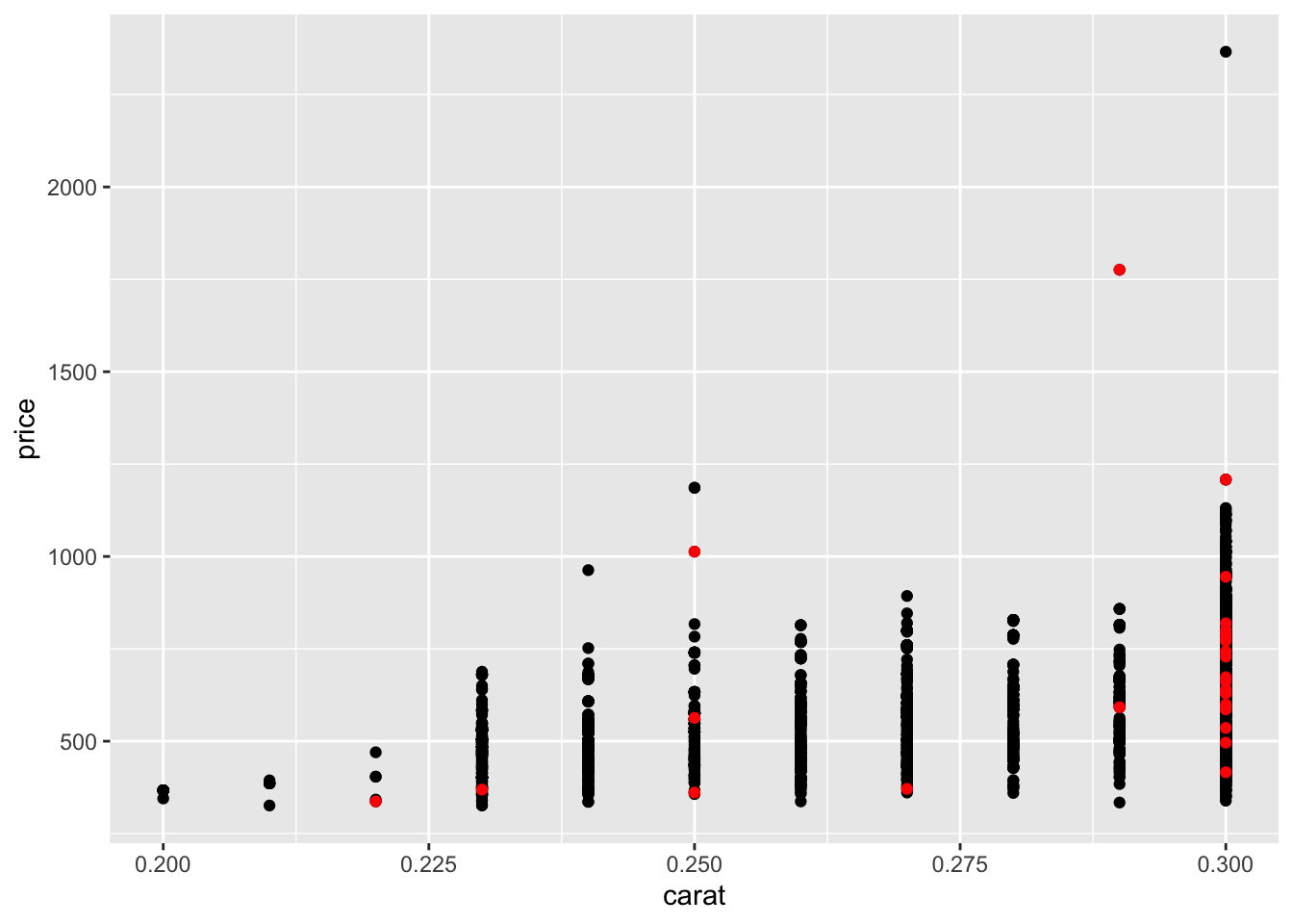
The placeholder even works at “later” points in a pipeline. We can use it to help simplify code, as you did above.