62 Model: Assessing Classification with ROC

Purpose: With regression models, we used model metrics in order to assess and select a model (e.g. choose which features we should use). In order to do the same with classification models, we need some quantitative measure of accuracy. However, assessing the “accuracy” of a classifier is far more complicated. To do this, we’ll need to understand the receiver operating characteristic.

Reading: StatQuest: ROC and AUC… clearly explained! (Required, ~17 minutes)

library(tidyverse)

## ── Attaching packages ─────────────────────────────────────── tidyverse 1.3.0 ──

## ✔ ggplot2 3.4.0      ✔ purrr   1.0.1 
## ✔ tibble  3.1.8      ✔ dplyr   1.0.10
## ✔ tidyr   1.2.1      ✔ stringr 1.5.0 
## ✔ readr   2.1.3      ✔ forcats 0.5.2

## ── Conflicts ────────────────────────────────────────── tidyverse_conflicts() ──
## ✖ dplyr::filter() masks stats::filter()
## ✖ dplyr::lag()    masks stats::lag()

library(modelr)
library(broom)

## 
## Attaching package: 'broom'

## The following object is masked from 'package:modelr':
## 
##     bootstrap

## We'll need the logit and inverse-logit functions to "warp space"
logit <- function(p) {
  odds_ratio <- p / (1 - p)
  log(odds_ratio)
}

inv.logit <- function(x) {
  exp(x) / (1 + exp(x))
}

62.1 Setup

Note: The following chunk contains a lot of stuff, but you already did this in e-model04-logistic!

## NOTE: No need to edit; you did all this in a previous exercise!
url_disease <- "http://archive.ics.uci.edu/ml/machine-learning-databases/heart-disease/processed.cleveland.data"
filename_disease <- "./data/uci_heart_disease.csv"

## Download the data locally
curl::curl_download(
        url_disease,
        destfile = filename_disease
      )

## Wrangle the data
col_names <- c(
  "age",
  "sex",
  "cp",
  "trestbps",
  "chol",
  "fbs",
  "restecg",
  "thalach",
  "exang",
  "oldpeak",
  "slope",
  "ca",
  "thal",
  "num"
)

## Recoding functions
convert_sex <- function(x) {
  case_when(
    x == 1 ~ "male",
    x == 0 ~ "female",
    TRUE ~ NA_character_
  )
}
convert_cp <- function(x) {
  case_when(
    x == 1 ~ "typical angina",
    x == 2 ~ "atypical angina",
    x == 3 ~ "non-anginal pain",
    x == 4 ~ "asymptomatic",
    TRUE ~ NA_character_
  )
}
convert_fbs <- function(x) {
  if_else(x == 1, TRUE, FALSE)
}
convert_restecv <- function(x) {
  case_when(
    x == 0 ~ "normal",
    x == 1 ~ "ST-T wave abnormality",
    x == 2 ~ "Estes' criteria",
    TRUE ~ NA_character_
  )
}
convert_exang <- function(x) {
  if_else(x == 1, TRUE, FALSE)
}
convert_slope <- function(x) {
  case_when(
    x == 1 ~ "upsloping",
    x == 2 ~ "flat",
    x == 3 ~ "downsloping",
    TRUE ~ NA_character_
  )
}
convert_thal <- function(x) {
  case_when(
    x == 3 ~ "normal",
    x == 6 ~ "fixed defect",
    x == 7 ~ "reversible defect",
    TRUE ~ NA_character_
  )
}

## Load and wrangle
df_data <-
  read_csv(
    filename_disease,
    col_names = col_names,
    col_types = cols(
      "age" = col_number(),
      "sex" = col_number(),
      "cp" = col_number(),
      "trestbps" = col_number(),
      "chol" = col_number(),
      "fbs" = col_number(),
      "restecg" = col_number(),
      "thalach" = col_number(),
      "exang" = col_number(),
      "oldpeak" = col_number(),
      "slope" = col_number(),
      "ca" = col_number(),
      "thal" = col_number(),
      "num" = col_number()
    )
  ) %>%
  mutate(
    sex = convert_sex(sex),
    cp = convert_cp(cp),
    fbs = convert_fbs(fbs),
    restecg = convert_restecv(restecg),
    exang = convert_exang(exang),
    slope = convert_slope(slope),
    thal = convert_thal(thal)
  ) %>%
  rowid_to_column() %>%
  ## Filter rows with NA's (you did this in e-data13-cleaning)
  filter(!is.na(ca), !is.na(thal)) %>%
  ## Create binary outcome for heart disease
  mutate(heart_disease = num > 0)

## Warning: One or more parsing issues, call `problems()` on your data frame for details,
## e.g.:
##   dat <- vroom(...)
##   problems(dat)

set.seed(101)

df_train <-
  df_data %>%
  slice_sample(n = 200)

df_validate <-
  anti_join(
    df_data,
    df_train,
    by = "rowid"
  )

62.2 Assessing a Classifier

What makes for a “good” or a “bad” classifier? When studying continuous models, we studied a variety of diagnostic plots and error metrics to assess model accuracy. However, since we’re now dealing with a discrete response, our metrics are going to look very different. In order to assess a classifier, we’re going to need to build up some concepts.

To learn these concepts, let’s return to the basic model from the previous modeling exercise:

## NOTE: No need to edit
## Fit a basic logistic regression model: biological-sex only
fit_basic <- glm(
  formula = heart_disease ~ sex,
  data = df_train,
  family = "binomial"
)

## Predict the heart disease probabilities on the validation data
df_basic <-
  df_validate %>%
  add_predictions(fit_basic, var = "log_odds_ratio") %>%
  arrange(log_odds_ratio) %>%
  rowid_to_column(var = "order") %>%
  mutate(pr_heart_disease = inv.logit(log_odds_ratio))

62.3 Positives and negatives

With a binary (two-class) classifier, there are only 4 possible outcomes of a single prediction. We can summarize all four in a table:

Note: A table with the total counts of [TP, FP, FN, TN] is called a confusion matrix.

There are two ways in which we can be correct:

True Positive: We correctly identified a positive case; e.g. we correctly identified that a given patient has heart disease.
True Negative: We correctly identified a negative case; e.g. we correctly identified that a given patient does not have heart disease.

And there are two ways in which we can be incorrect:

False Positive: We predicted a case to be positive, but in reality it was negative; e.g. we predicted that a given patient has heart disease, but in reality they do not have the disease.
False Negative: We predicted a case to be negative, but in reality it was positive; e.g. we predicted that a given patient does not have heard disease, but in reality they do have the disease.

Note that we might have different concerns about false positives and negatives. For instance in the heart disease case, we might be more concerned with flagging all possible cases of heart disease, particularly if follow-up examination can diagnose heart disease with greater precision. In that case, we might want to avoid false negatives but accept more false positives.

We can make quantitative judgments about these classification tradeoffs by controlling classification rates with a decision threshold.

62.4 Classification Rates and Decision Thresholds

We can summarize the tradeoffs a classifier makes in terms of classification rates. First, let’s introduce some shorthand:

TP | Total count of True Positives |
FP | Total count of False Positives |
TN | Total count of True Negatives |
FN | Total count of False Negatives |

Two important rates are the true positive rate and false positive rate, defined as:

True Positive Rate (TPR): The ratio of true positives to all positives, that is:

TPR = TP / P = TP / (TP + FN)

We generally want to maximize the TPR. In the heart disease example, this is the number of patients with heart disease that we correctly diagnose; a higher TPR in this setting means we can follow-up with and treat more individuals.

False Positive Rate (FPR): The ratio of false positives to all negatives, that is:

FPR = FP / N = FP / (FP + TN)

We generally want to minimize the FPR. In the heart disease example, this is the number of patients without heart disease that we falsely diagnose with the disease; a higher FPR in this setting means we will waste valuable time and resources following up with healthy individuals.

We can control the TPR and FPR by choosing our decision threshold for our classifier. Remember that in the previous exercise e-model04-logistic we set an arbitrary threshold of pr_heart_disease > 0.5 for detection: We can instead pick a pr_threshold to make our classifier more or less sensitive, which will adjust the TPR and FPR. The next task will illustrate this idea.

62.4.1 q1 Compute the true positive rate (TPR) and false positive rate (FPR) using the model fitted above, calculating on the validation data.

Hint 1: Remember that you can use summarize(n = sum(boolean)) to count the number of TRUE values in a variable boolean. Feel free to compute intermediate boolean values with things like mutate(boolean = (x < 0) & flag) before your summarize.

Hint 2: We did part of this in the previous modeling exercise!

pr_threshold <- 0.5

df_q1 <-
  df_basic %>%
  mutate(
    true_positive = (pr_heart_disease > pr_threshold) & heart_disease,
    false_positive = (pr_heart_disease > pr_threshold) & !heart_disease,
    true_negative = (pr_heart_disease <= pr_threshold) & !heart_disease,
    false_negative = (pr_heart_disease <= pr_threshold) & heart_disease
  ) %>%
  summarize(
    TP = sum(true_positive),
    FP = sum(false_positive),
    TN = sum(true_negative),
    FN = sum(false_negative)
  ) %>%
  mutate(
    TPR = TP / (TP + FN),
    FPR = FP / (FP + TN)
  )

df_q1

## # A tibble: 1 × 6
##      TP    FP    TN    FN   TPR   FPR
##   <int> <int> <int> <int> <dbl> <dbl>
## 1    26    37    24    10 0.722 0.607

Use the following test to check your work.

## NOTE: No need to edit; use this to check your work
assertthat::assert_that(
  all_equal(
    df_q1 %>% select(TPR, FPR),
    df_validate %>%
      add_predictions(fit_basic, var = "l_heart_disease") %>%
      mutate(pr_heart_disease = inv.logit(l_heart_disease)) %>%
    summarize(
      TP = sum((pr_heart_disease > pr_threshold) & heart_disease),
      FP = sum((pr_heart_disease > pr_threshold) & !heart_disease),
      TN = sum((pr_heart_disease <= pr_threshold) & !heart_disease),
      FN = sum((pr_heart_disease <= pr_threshold) & heart_disease)
    ) %>%
    mutate(
      TPR = TP / (TP + FN),
      FPR = FP / (FP + TN)
    ) %>%
    select(TPR, FPR)
  )
)

## [1] TRUE

print("Excellent!")

## [1] "Excellent!"

62.5 The Receiver Operating Characteristic (ROC) Curve

As the required video mentioned, we can summarize TPR and FPR at different threshold values pr_threshold with the receiver operating characteristic curve (ROC curve). This plot gives us an overview of the tradeoffs we can achieve with our classification model.

The ROC curve shows TPR against FPR. Remember that we want to maximize TPR and minimize FPR*; therefore, the ideal point for the curve to reach is the top-left point in the graph. A very poor classifier would run along the diagonal—this would be equivalent to randomly guessing the class of each observation. An ROC curve below the diagonal is worse than random guessing!

To compute an ROC curve, we could construct a confusion matrix at a variety of thresholds, compute the TPR and FPR for each, and repeat. However, there’s a small bit of “shortcut code” we could use to do the same thing. The following chunk illustrates how to compute an ROC curve.

62.5.1 q2 Inspect the following ROC curve for the basic classifier and assess its performance. Is this an effective classifier? How do you know?

## NOTE: No need to edit; run and inspect
df_basic %>%
  ## Begin: Shortcut code for computing an ROC
  arrange(desc(pr_heart_disease)) %>%
  summarize(
    true_positive_rate = cumsum(heart_disease) / sum(heart_disease),
    false_positive_rate = cumsum(!heart_disease) / sum(!heart_disease)
  ) %>%
  ## End: Shortcut code for computing an ROC

  ggplot(aes(false_positive_rate, true_positive_rate)) +
  geom_abline(intercept = 0, slope = 1, linetype = 2) +
  geom_step() +
  coord_cartesian(xlim = c(0, 1), ylim = c(0, 1)) +
  theme_minimal()

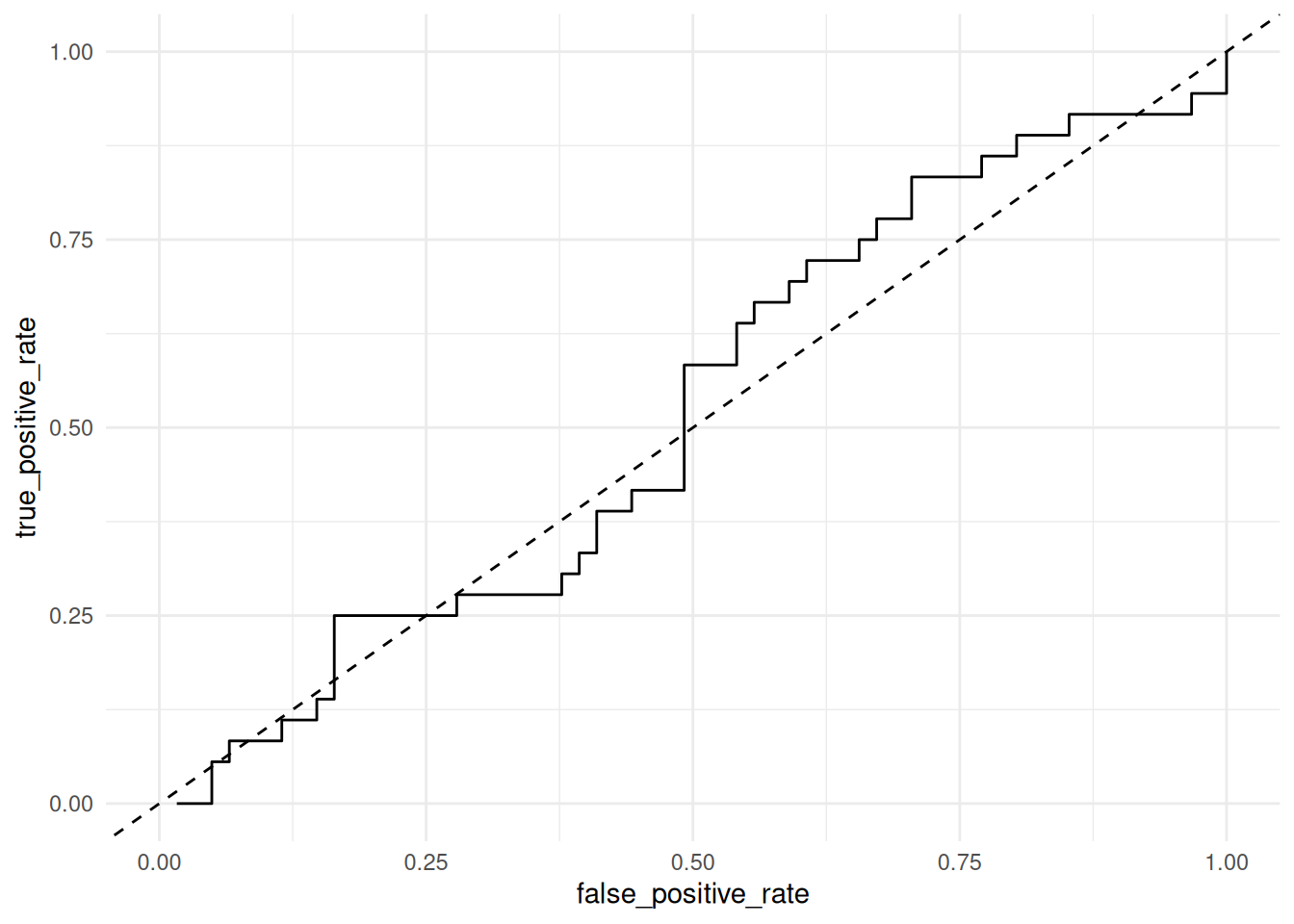
Observations:

This is a highly ineffective classifier; the ROC curve is very near the diagonal, indicating the classifier is not much better (for some thresholds—worse than) random guessing.

62.6 Practice Assessing Classifiers

Let’s get some practice reading ROC curves.

62.6.1 q3 Inspect the following ROC curve. Is this an effective classifier? What explains this model’s performance? Is this model valid for prediction?

## NOTE: No need to edit
fit_cheating <- glm(
  formula = heart_disease ~ num,
  data = df_train,
  family = "binomial"
)

## Warning: glm.fit: algorithm did not converge

## Warning: glm.fit: fitted probabilities numerically 0 or 1 occurred

df_cheating <-
  df_validate %>%
  add_predictions(fit_cheating, var = "log_odds_ratio") %>%
  arrange(log_odds_ratio) %>%
  rowid_to_column(var = "order") %>%
  mutate(pr_heart_disease = inv.logit(log_odds_ratio))

df_cheating %>%
  ## Begin: Shortcut code for computing an ROC
  arrange(desc(pr_heart_disease)) %>%
  summarize(
    true_positive_rate = cumsum(heart_disease) / sum(heart_disease),
    false_positive_rate = cumsum(!heart_disease) / sum(!heart_disease)
  ) %>%
  ## End: Shortcut code for computing an ROC

  ggplot(aes(false_positive_rate, true_positive_rate)) +
  geom_abline(intercept = 0, slope = 1, linetype = 2) +
  geom_step() +
  coord_cartesian(xlim = c(0, 1), ylim = c(0, 1)) +
  theme_minimal()

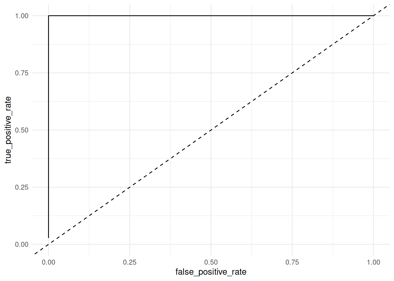
Observations:

This is an optimal classifier; we can achieve TPR = 1 with FPR = 0. In fact, it’s suspiciously good….
This model is using the outcome to predict the outcome! Remember that heart_disease = num > 0; this is not a valid way to predict the presence of heart disease.

Next you’ll fit your own model and assess its performance.

62.6.2 q4 Fit a model to the training data, and predict class probabilities on the validation data. Compare your model’s performance to that of `fit_baseline` (fitted below).

fit_q4 <- glm(
  formula = heart_disease ~ age + cp + trestbps,
  data = df_train,
  family = "binomial"
)

df_q4 <-
  df_validate %>%
  add_predictions(fit_q4, var = "log_odds_ratio") %>%
  arrange(log_odds_ratio) %>%
  rowid_to_column(var = "order") %>%
  mutate(pr_heart_disease = inv.logit(log_odds_ratio))

## Here's another model for comparison
fit_baseline <- glm(
  formula = heart_disease ~ sex + cp + trestbps,
  data = df_train,
  family = "binomial"
)

df_baseline <-
  df_validate %>%
  add_predictions(fit_baseline, var = "log_odds_ratio") %>%
  arrange(log_odds_ratio) %>%
  rowid_to_column(var = "order") %>%
  mutate(pr_heart_disease = inv.logit(log_odds_ratio))

## NOTE: No need to edit
bind_rows(
  df_q4 %>%
    arrange(desc(pr_heart_disease)) %>%
    summarize(
      true_positive_rate = cumsum(heart_disease) / sum(heart_disease),
      false_positive_rate = cumsum(!heart_disease) / sum(!heart_disease)
    ) %>%
    mutate(model = "Personal"),
  df_baseline %>%
    arrange(desc(pr_heart_disease)) %>%
    summarize(
      true_positive_rate = cumsum(heart_disease) / sum(heart_disease),
      false_positive_rate = cumsum(!heart_disease) / sum(!heart_disease)
    ) %>%
    mutate(model = "Baseline")
  ) %>%

  ggplot(aes(false_positive_rate, true_positive_rate, color = model)) +
  geom_abline(intercept = 0, slope = 1, linetype = 2) +
  geom_step() +
  coord_cartesian(xlim = c(0, 1), ylim = c(0, 1)) +
  theme_minimal() +
  theme(legend.position = "bottom")

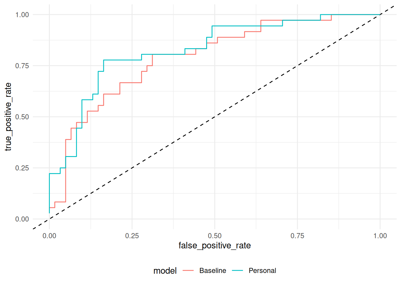
Observations:

My model fit_q4 is comparable in performance to fit_baseline; it outperforms (in TPR for fixed FPR) in some places, and underperforms in others.
As one sweeps from low to high FPR, the TPR increases—at first quickly, then it tapers off to increase slowly. Both FPR and TPR equal zero at the beginning, and both limit to one. The “tradeoff” is that we can have an arbitrarily high TPR, but we “pay” for this through an increase in the FPR.

62.7 Selecting a Threshold

The ROC summarizes performance characteristics for a variety of thresholds pr_threshold, but to actually deploy a classifier and make decisions, we have to pick a specific threshold value. Picking a threshold is not just an exercise in mathematics; we need to inform this decision with our intended use-case.

The following chunk plots potential pr_threshold against achieved TPR values for your model. Use this image to pick a classifier threshold.

62.7.1 q5 Pick a target TPR value for your heart disease predictor; what is a reasonable value for `TPR`, and why did yo pick that value? What values of `pr_threshold` meet or exceed that target TPR? What specific value for `pr_threshold` do you choose, and why?

## NOTE: No need to edit this; use these data to pick a threshold
df_thresholds <-
  df_q4 %>%
  ## Begin: Shortcut code for computing an ROC
  arrange(desc(pr_heart_disease)) %>%
  summarize(
    pr_heart_disease = pr_heart_disease,
    true_positive_rate = cumsum(heart_disease) / sum(heart_disease),
    false_positive_rate = cumsum(!heart_disease) / sum(!heart_disease)
  )
  ## End: Shortcut code for computing an ROC

## TODO: Pick a threshold using df_thresholds above
df_thresholds %>%
  filter(true_positive_rate >= 0.9) %>%
  filter(false_positive_rate == min(false_positive_rate))

## # A tibble: 2 × 3
##   pr_heart_disease true_positive_rate false_positive_rate
##              <dbl>              <dbl>               <dbl>
## 1            0.252              0.917               0.492
## 2            0.249              0.944               0.492

pr_threshold <- 0.249
tpr_achieved <- 0.944
fpr_achieved <- 0.492

## NOTE: No need to edit; use this visual to help your decision
df_thresholds %>%
  ggplot(aes(true_positive_rate, pr_heart_disease)) +
  geom_vline(xintercept = tpr_achieved, linetype = 2) +
  geom_hline(yintercept = pr_threshold, linetype = 2) +
  geom_step() +
  labs(
    x = "True Positive Rate",
    y = "Pr Threshold"
  )

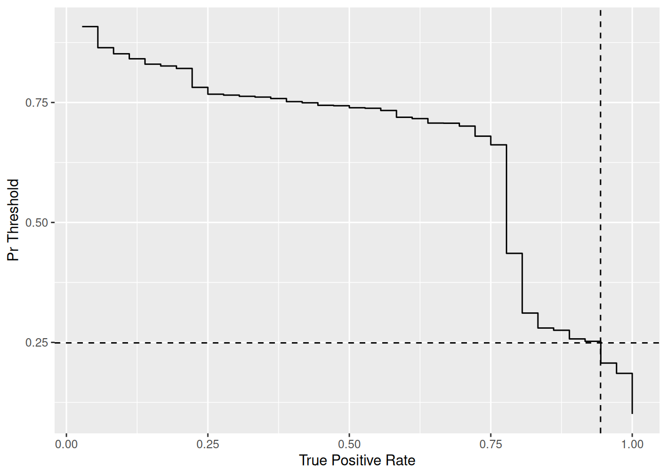
Observations:

I pick TPR > 0.9, as I want to catch the vast majority of patients with the disease.
Filtering df_thresholds shows that pr_threshold >= 0.252 achieves my desired TPR.
To pick a specific value for pr_threshold, I also try to minimize the FPR. For my case, there is a range of values of pr_threshold that can minimize the FPR; therefore I take the more permissive end of the interval.
Ultimately I picked pr_threshold = 0.249, which gave TPR = 0.944, FPR = 0.492. This will lead to a lot of false positives, but we will have a very sensitive detector.

62 Model: Assessing Classification with ROC

62.1 Setup

62.2 Assessing a Classifier

62.3 Positives and negatives

62.4 Classification Rates and Decision Thresholds

62.4.1 q1 Compute the true positive rate (TPR) and false positive rate (FPR) using the model fitted above, calculating on the validation data.

62.5 The Receiver Operating Characteristic (ROC) Curve

62.5.1 q2 Inspect the following ROC curve for the basic classifier and assess its performance. Is this an effective classifier? How do you know?

62.6 Practice Assessing Classifiers

62.6.1 q3 Inspect the following ROC curve. Is this an effective classifier? What explains this model’s performance? Is this model valid for prediction?

62.6.2 q4 Fit a model to the training data, and predict class probabilities on the validation data. Compare your model’s performance to that of fit_baseline (fitted below).

62.7 Selecting a Threshold

62.7.1 q5 Pick a target TPR value for your heart disease predictor; what is a reasonable value for TPR, and why did yo pick that value? What values of pr_threshold meet or exceed that target TPR? What specific value for pr_threshold do you choose, and why?

62.6.2 q4 Fit a model to the training data, and predict class probabilities on the validation data. Compare your model’s performance to that of `fit_baseline` (fitted below).

62.7.1 q5 Pick a target TPR value for your heart disease predictor; what is a reasonable value for `TPR`, and why did yo pick that value? What values of `pr_threshold` meet or exceed that target TPR? What specific value for `pr_threshold` do you choose, and why?