42 Stats: Error and Bias

Purpose: Error is a subtle concept. Often statistics concepts are introduced with a host of assumptions on the errors. In this short exercise, we’ll reminder ourselves what errors are and learn what happens when one standard assumption—unbiasedness—is violated.

Prerequisites: c02-michelson, e-stat06-clt

## Note: No need to edit this chunk!
library(tidyverse)

## ── Attaching packages ─────────────────────────────────────── tidyverse 1.3.0 ──

## ✔ ggplot2 3.4.0      ✔ purrr   1.0.1 
## ✔ tibble  3.1.8      ✔ dplyr   1.0.10
## ✔ tidyr   1.2.1      ✔ stringr 1.5.0 
## ✔ readr   2.1.3      ✔ forcats 0.5.2

## ── Conflicts ────────────────────────────────────────── tidyverse_conflicts() ──
## ✖ dplyr::filter() masks stats::filter()
## ✖ dplyr::lag()    masks stats::lag()

library(googlesheets4)

url <- "https://docs.google.com/spreadsheets/d/1av_SXn4j0-4Rk0mQFik3LLr-uf0YdA06i3ugE6n-Zdo/edit?usp=sharing"

c_true <- 299792.458 # Exact speed of light in a vacuum (km / s)
c_michelson <- 299944.00  # Michelson's speed estimate (km / s)

meas_adjust <- +92 # Michelson's speed of light adjustment (km / s)
c_michelson_uncertainty <- 51 # Michelson's measurement uncertainty (km / s)

gs4_deauth()
ss <- gs4_get(url)
df_michelson <-
  read_sheet(ss) %>%
  select(Date, Distinctness, Temp, Velocity) %>%
  mutate(
    Distinctness = as_factor(Distinctness),
    c_meas = Velocity + meas_adjust
  )

## ✔ Reading from "michelson1879".

## ✔ Range 'Sheet1'.

42.1 Errors

Let’s re-examine the Michelson speed of light data to discuss the concept of error. Let \(c\) denote the true speed of light, and let \(\hat{c}_i\) denote the i-th measurement by Michelson. Then the error \(\epsilon_{c,i}\) is:

\[\epsilon_{c,i} \equiv \hat{c}_i - c.\]

Note that these are errors (and not some other quantity) because they are differences against the true value \(c\). Very frequently in statistics, we assume that the errors are unbiased; that is we assume \(\mathbb{E}[\epsilon] = 0\). Let’s take a look at what happens when that assumption is violated.

42.1.1 q1 Compute the errors \(\epsilon_c\) using Michelson’s measurements c_meas and the true speed of light c_true.

## TASK: Compute `epsilon_c`
df_q1 <-
  df_michelson %>%
  mutate(epsilon_c = c_meas - c_true)

df_q1 %>%
  ggplot(aes(epsilon_c)) +
  geom_histogram()

## `stat_bin()` using `bins = 30`. Pick better value with `binwidth`.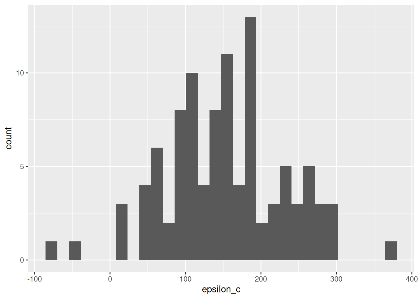

We can use descriptive statistics in order to summarize the errors. This will give us a quantification of the uncertainty in our measurements: remember that uncertainty is our assessment of the error.

42.1.2 q2 Estimate the mean and standard deviation of \(\epsilon_c\) from df_q1. Is the error mean large or small, compared to its standard deviation? How about compared to Michelson’s uncertainty c_michelson_uncertainty?

## TASK: Estimate `epsilon_mean` and `epsilon_sd` from df_q1
df_q2 <-
  df_q1 %>%
  summarize(
    epsilon_mean = mean(epsilon_c),
    epsilon_sd = sd(epsilon_c)
  )

Observations:

Use the following tests to check your answers.

## NOTE: No need to change this!
assertthat::assert_that(abs((df_q2 %>% pull(epsilon_mean)) - 151.942) < 1e-3)

## [1] TRUE

assertthat::assert_that(abs((df_q2 %>% pull(epsilon_sd)) - 79.01055) < 1e-3)

## [1] TRUE

print("Great job!")

## [1] "Great job!"

Generally, we want our errors to have zero mean—the case where the errors have zero mean is called unbiased. The quantity \(\mathbb{E}[\epsilon]\) is called bias, and an estimate such as \(\hat{c}\) with \(\mathbb{E}[\epsilon] \neq 0\) is called biased.

What can happen when our estimates are biased? In that case, increased data may not improve our estimate, and our statistical tools—such as confidence intervals—may give us a false impression of the true error. The next example will show us what happens if we apply confidence intervals in a biased-data setting like Michelson’s data.

42.1.3 q3 Use a CLT approximation to construct a \(99%\) confidence interval on the mean of c_meas. Check (with the provided code) if your CI includes the true speed of light.

Hint: This computation should not use the true speed of light \(c_true\) in any way.

## TASK: Compute a 99% confidence interval on the mean of c_meas
C <- 0.99
q <- qnorm( 1 - (1 - C) / 2 )
df_q3 <-
  df_q1 %>%
  summarize(
    c_meas_mean = mean(c_meas),
    c_meas_sd = sd(c_meas),
    n_samp = n(),
    c_lo = c_meas_mean - q * c_meas_sd / sqrt(n_samp),
    c_hi = c_meas_mean + q * c_meas_sd / sqrt(n_samp)
  )

## NOTE: This checks if the CI contains c_true
(df_q3 %>% pull(c_lo) <= c_true) & (c_true <= df_q3 %>% pull(c_hi))

## [1] FALSE

Use the following tests to check your answers.

## NOTE: No need to change this!
assertthat::assert_that(abs((df_q3 %>% pull(c_lo)) - 299924.048) < 1e-3)

## [1] TRUE

assertthat::assert_that(abs((df_q3 %>% pull(c_hi)) - 299964.752) < 1e-3)

## [1] TRUE

print("Well done!")

## [1] "Well done!"

Once you correctly compute a CI for c_meas, you should find that the interval does not include c_true. CI is never guaranteed to include its true value—it is a probabilistic construction, after all. However, we saw above that the errors are biased; even if we were to gather more data, our confidence intervals would converge on the wrong value. Statistics are not a cure-all!