10 Communication: Code Style
Purpose: From the tidyverse style guide “Good coding style is like correct punctuation: you can manage without it, butitsuremakesthingseasiertoread.” We will follow the tidyverse style guide; Google’s internal R style guide is actually based on these guidelines!
Reading: tidyverse style guide. Topics: Spacing (subsection only), Pipes (whole section) Reading Time: ~ 10 minutes
## ── Attaching core tidyverse packages ──────────────────────── tidyverse 2.0.0 ──
## ✔ dplyr     1.1.4     ✔ readr     2.1.5
## ✔ forcats   1.0.0     ✔ stringr   1.5.1
## ✔ ggplot2   3.5.2     ✔ tibble    3.2.1
## ✔ lubridate 1.9.4     ✔ tidyr     1.3.1
## ✔ purrr     1.0.4
## ── Conflicts ────────────────────────────────────────── tidyverse_conflicts() ──
## ✖ dplyr::filter() masks stats::filter()
## ✖ dplyr::lag()    masks stats::lag()
## ℹ Use the conflicted package (<http://conflicted.r-lib.org/>) to force all conflicts to become errors
10.0.1 q1 Re-write according to the style guide
Hint: The pipe operator %>% will help make this code more readable.
## # A tibble: 5 × 2
##   cut       mean_price
##   <ord>          <dbl>
## 1 Fair           4359.
## 2 Good           3929.
## 3 Very Good      3982.
## 4 Premium        4584.
## 5 Ideal 3458.## # A tibble: 5 × 2
## cut mean_price
## <ord> <dbl>
## 1 Fair 4359.
## 2 Good 3929.
## 3 Very Good 3982.
## 4 Premium 4584.
## 5 Ideal 3458.10.0.2 q2 Re-write according to the style guide
Hint: There are particular rules about spacing!
## NOTE: You can copy this code to the chunk below
iris %>%
  mutate(Sepal.Area=Sepal.Length*Sepal.Width) %>%
  group_by( Species ) %>%
  summarize_if(is.numeric,mean)%>%
  ungroup() %>%
  pivot_longer( names_to="measure",values_to="value",cols=-Species ) %>%
  arrange(value )
## # A tibble: 15 × 3
## Species measure value
## <fct> <chr> <dbl>
## 1 setosa Petal.Width 0.246
## 2 versicolor Petal.Width 1.33
## 3 setosa Petal.Length 1.46
## 4 virginica Petal.Width 2.03
## 5 versicolor Sepal.Width 2.77
## 6 virginica Sepal.Width 2.97
## 7 setosa Sepal.Width 3.43
## 8 versicolor Petal.Length 4.26
## 9 setosa Sepal.Length 5.01
## 10 virginica Petal.Length 5.55
## 11 versicolor Sepal.Length 5.94
## 12 virginica Sepal.Length 6.59
## 13 versicolor Sepal.Area 16.5
## 14 setosa Sepal.Area 17.3
## 15 virginica Sepal.Area 19.7iris %>%
mutate(Sepal.Area = Sepal.Length * Sepal.Width) %>%
group_by(Species) %>%
summarize_if(is.numeric, mean) %>%
ungroup() %>%
pivot_longer(names_to = "measure", values_to = "value", cols = -Species) %>%
arrange(value)## # A tibble: 15 × 3
## Species measure value
## <fct> <chr> <dbl>
## 1 setosa Petal.Width 0.246
## 2 versicolor Petal.Width 1.33
## 3 setosa Petal.Length 1.46
## 4 virginica Petal.Width 2.03
## 5 versicolor Sepal.Width 2.77
## 6 virginica Sepal.Width 2.97
## 7 setosa Sepal.Width 3.43
## 8 versicolor Petal.Length 4.26
## 9 setosa Sepal.Length 5.01
## 10 virginica Petal.Length 5.55
## 11 versicolor Sepal.Length 5.94
## 12 virginica Sepal.Length 6.59
## 13 versicolor Sepal.Area 16.5
## 14 setosa Sepal.Area 17.3
## 15 virginica Sepal.Area 19.710.0.3 q3 Re-write according to the style guide
Hint: What do we do about long lines?
iris %>%
  group_by(Species) %>%
  summarize(Sepal.Length = mean(Sepal.Length), Sepal.Width = mean(Sepal.Width), Petal.Length = mean(Petal.Length), Petal.Width = mean(Petal.Width))
## # A tibble: 3 × 5
## Species Sepal.Length Sepal.Width Petal.Length Petal.Width
## <fct> <dbl> <dbl> <dbl> <dbl>
## 1 setosa 5.01 3.43 1.46 0.246
## 2 versicolor 5.94 2.77 4.26 1.33
## 3 virginica 6.59 2.97 5.55 2.03iris %>%
group_by(Species) %>%
summarize(
Sepal.Length = mean(Sepal.Length),
Sepal.Width = mean(Sepal.Width),
Petal.Length = mean(Petal.Length),
Petal.Width = mean(Petal.Width)
)## # A tibble: 3 × 5
## Species Sepal.Length Sepal.Width Petal.Length Petal.Width
## <fct> <dbl> <dbl> <dbl> <dbl>
## 1 setosa 5.01 3.43 1.46 0.246
## 2 versicolor 5.94 2.77 4.26 1.33
## 3 virginica 6.59 2.97 5.55 2.03The following is an addition I’m making to the “effective styleguide” for the class: Rather than doing this:

Instead, do this:
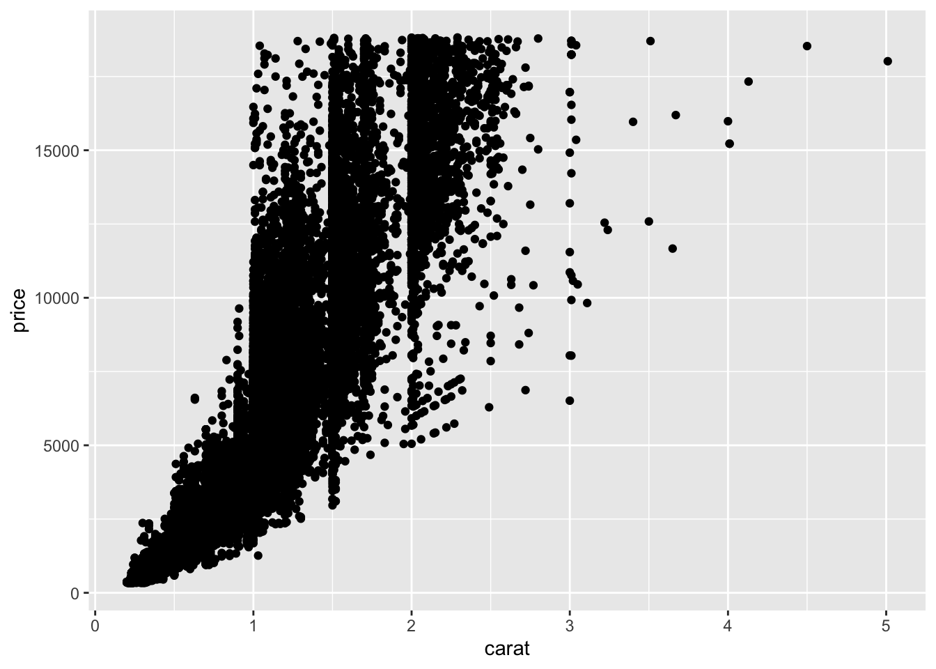
This may seem like a small difference (it is), but getting in this habit will pay off when we start combining data operations with plotting; for instance:
## NOTE: No need to edit, just an example
diamonds %>%
  filter(1.5 <= carat, carat <= 2.0) %>%

  ggplot(aes(carat, price)) +
  geom_point()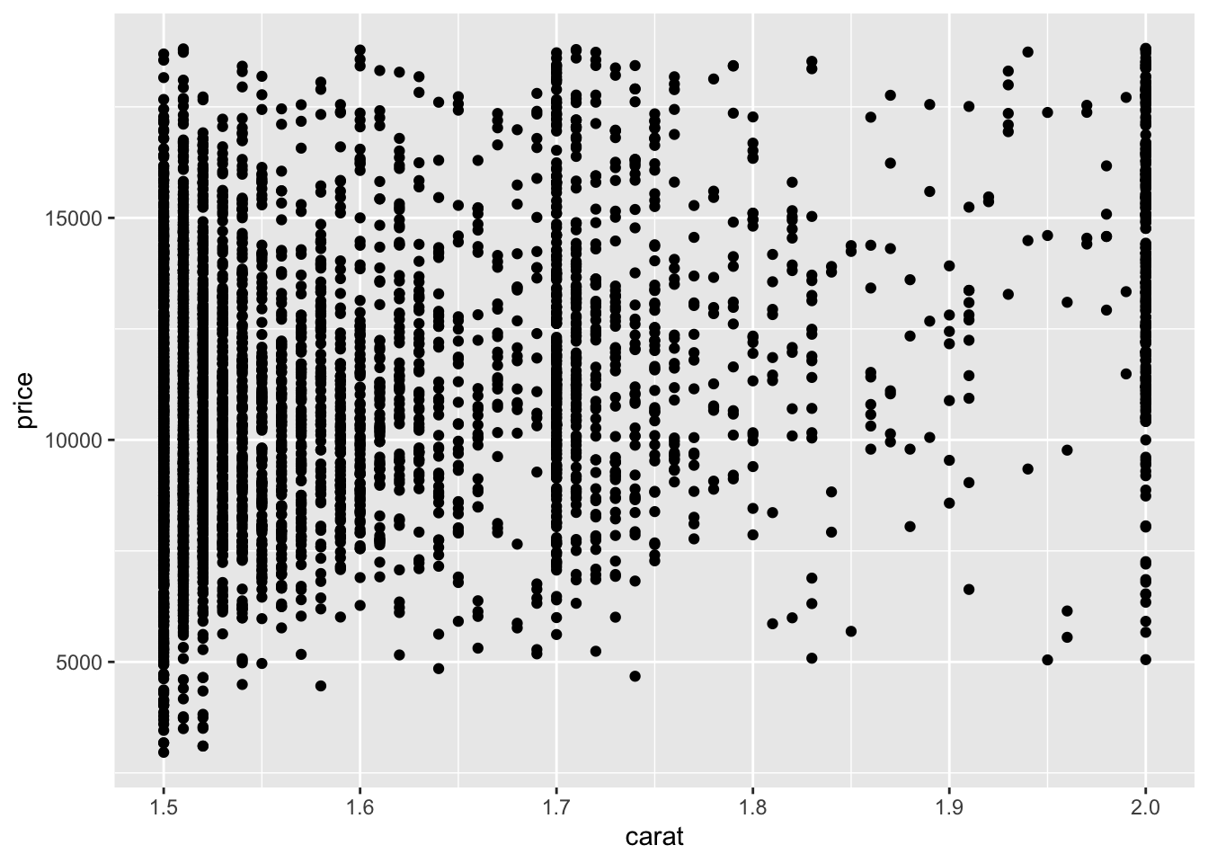
Getting in the habit of “putting the data first” will make it easier for you to add preprocessing steps. Also, you can easily “disable” the plot to inspect your preprocessing while debugging; that is:
## NOTE: No need to edit, just an example
diamonds %>%
  filter(1.5 <= carat, carat <= 2.0) %>%
  glimpse()
## Rows: 4,346
## Columns: 10
## $ carat <dbl> 1.50, 1.52, 1.52, 1.50, 1.50, 1.50, 1.51, 1.52, 1.52, 1.50, 1.…
## $ cut <ord> Fair, Good, Good, Fair, Good, Premium, Good, Fair, Premium, Pr…
## $ color <ord> H, E, E, H, G, H, G, H, I, H, I, F, F, I, H, D, G, F, H, H, E,…
## $ clarity <ord> I1, I1, I1, I1, I1, I1, I1, I1, I1, I1, I1, I1, I1, I1, I1, I1…
## $ depth <dbl> 65.6, 57.3, 57.3, 69.3, 57.4, 60.1, 64.0, 64.9, 61.2, 61.1, 63…
## $ table <dbl> 54, 58, 58, 61, 62, 57, 59, 58, 58, 59, 61, 59, 56, 58, 61, 60…
## $ price <int> 2964, 3105, 3105, 3175, 3179, 3457, 3497, 3504, 3541, 3599, 36…
## $ x <dbl> 7.26, 7.53, 7.53, 6.99, 7.56, 7.40, 7.29, 7.18, 7.43, 7.37, 7.…
## $ y <dbl> 7.09, 7.42, 7.42, 6.81, 7.39, 7.28, 7.17, 7.13, 7.35, 7.26, 7.…
## $ z <dbl> 4.70, 4.28, 4.28, 4.78, 4.29, 4.42, 4.63, 4.65, 4.52, 4.47, 4.…I’ll enforce this “data first” style, but after this class you are (of course) free to write code however you like!
10.0.4 q4 Re-write according to the style guide
Hint: Put the data first!
ggplot(
  iris %>%
  pivot_longer(
    names_to = c("Part", ".value"),
    names_sep = "\\.",
    cols = -Species
  ),
  aes(Width, Length, color = Part)
) +
  geom_point() +
  facet_wrap(~Species)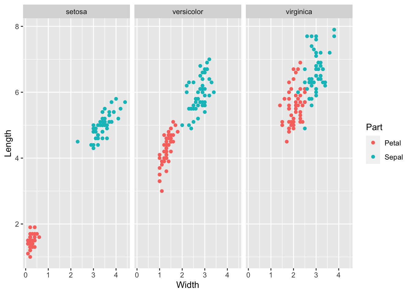
iris %>%
  pivot_longer(
    names_to = c("Part", ".value"),
    names_sep = "\\.",
    cols = -Species
  ) %>%

  ggplot(aes(Width, Length, color = Part)) +
  geom_point() +
  facet_wrap(~Species)