55 Model: Model Selection and the Test-Validate Framework
Purpose: When designing a model, we need to make choices about the model form. However, since we are optimizing the model to fit our data, we need to be careful not to bias our assessments and make poor modeling choices. We can use a training and validation split of our data to help make these choices. To understand these issues, we’ll discuss underfitting, overfitting, and the test-validate framework.
Reading: Training, validation, and test sets (Optional)
## ── Attaching core tidyverse packages ──────────────────────── tidyverse 2.0.0 ──
## ✔ dplyr     1.1.4     ✔ readr     2.1.5
## ✔ forcats   1.0.0     ✔ stringr   1.5.1
## ✔ ggplot2   3.5.2     ✔ tibble    3.2.1
## ✔ lubridate 1.9.4     ✔ tidyr     1.3.1
## ✔ purrr     1.0.4
## ── Conflicts ────────────────────────────────────────── tidyverse_conflicts() ──
## ✖ dplyr::filter() masks stats::filter()
## ✖ dplyr::lag()    masks stats::lag()
## ℹ Use the conflicted package (<http://conflicted.r-lib.org/>) to force all conflicts to become errors##
## Attaching package: 'broom'
##
## The following object is masked from 'package:modelr':
##
## bootstrapWe’ll look at two cases: First a simple problem studying polynomials, then a more realistic case using the diamonds dataset.
55.1 Illustrative Case: Polynomial Regression
To illustrate the ideas behind the test-validate framework, let’s study a very simple problem: Fitting a polynomial. The following code sets up this example.
## NOTE: No need to edit this chunk
set.seed(101)

# Ground-truth function we seek to approximate
fcn_true <- function(x) {12 * (x - 0.5)^3 - 2 * x + 1}

# Generate data
n_samples <- 100
df_truth <-
  tibble(x = seq(0, 1, length.out = n_samples)) %>%
  mutate(
    y = fcn_true(x),                     # True values
    y_meas = y + 0.05 * rnorm(n_samples) # Measured with noise
  )

# Select training data
df_measurements <-
  df_truth %>%
  slice_sample(n = 20) %>%
  select(x, y_meas)

# Visualize
df_truth %>%
  ggplot(aes(x, y)) +
  geom_line() +
  geom_point(
    data = df_measurements,
    mapping = aes(y = y_meas, color = "Measurements")
  )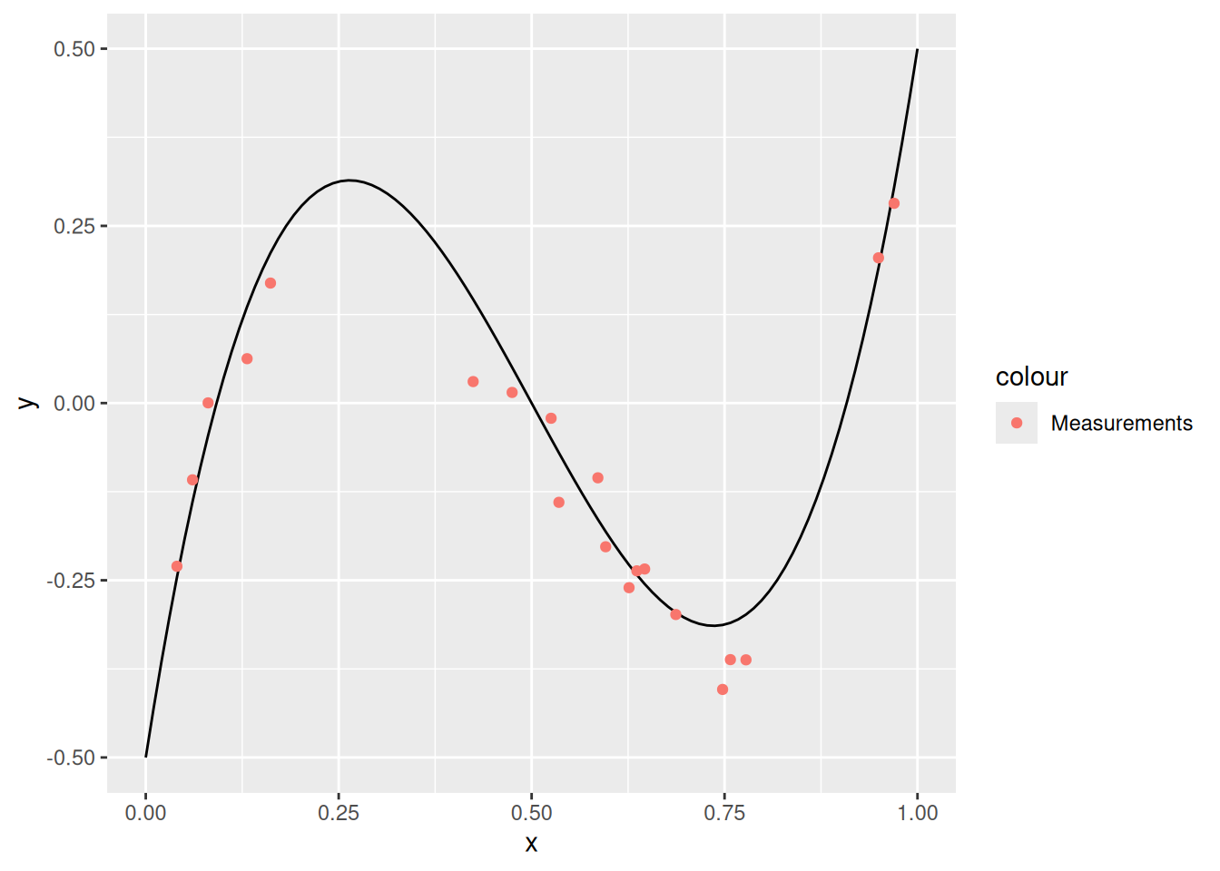
In what follows, we will behave as though we only have access to df_measurements—this is to model a “real” case where we have limited data. We will attempt to fit a polynomial to the data; remember that a polynomial of degree \(d\) is a function of the form
\[f_{\text{polynomial}}(x) = \sum_{i=0}^d \beta_i x^i,\]
where the \(\beta_i\) are coefficients, and \(x^0 = 1\) is a constant.
55.2 Underfitting
The following code fits a polynomial of degree 2 to the available data df_measurements.
55.2.1 q1 Run the following code and inspect the (visual) results. Describe whether the model (Predicted) captures the “trends” in the measured data (black dots).
## NOTE: No need to edit this code; run and inspect
# Fit a polynomial of degree = 2
fit_d2 <-
  df_measurements %>%
  lm(
    data = .,
    formula = y_meas ~ poly(x, degree = 2)
  )

# Visualize the results
df_truth %>%
  add_predictions(fit_d2, var = "y_pred") %>%

  ggplot(aes(x)) +
  geom_line(aes(y = y, color = "True")) +
  geom_line(aes(y = y_pred, color = "Predicted")) +
  geom_point(data = df_measurements, aes(y = y_meas)) +

  scale_color_discrete(name = "") +
  theme_minimal()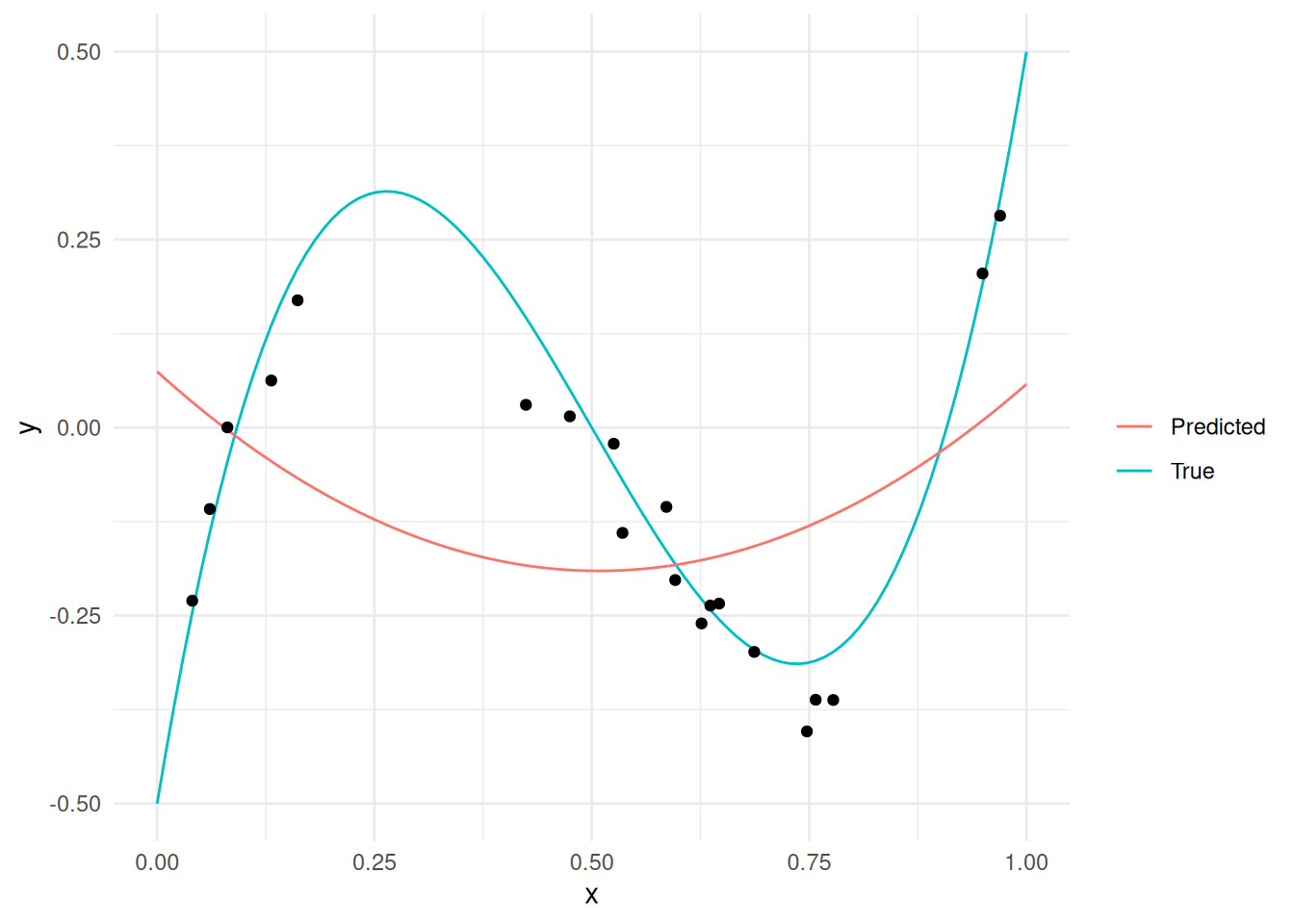
Observations:
- The
Predictedvalues do not capture the trend in the measured points, nor in theTruefunction.
This phenomenon is called underfitting: This is when the model is not “flexible” enough to capture trends observed in the data. We can increase the flexibility of the model by increasing the polynomial order, which we’ll do below.
55.3 Overfitting
Let’s increase the polynomial order and re-fit the data to try to solve the underfitting problem.
55.3.1 q2 Copy the code from above to fit a degree = 17 polynomial to the measurements.
## TASK: Fit a high-degree polynomial to df_measurements
fit_over <-
  df_measurements %>%
  lm(data = ., formula = y_meas ~ poly(x, degree = 17))

## NOTE: No need to modify code below
y_limits <-
  c(
    df_truth %>% pull(y) %>% min(),
    df_truth %>% pull(y) %>% max()
  )

df_truth %>%
  add_predictions(fit_over, var = "y_pred") %>%

  ggplot(aes(x)) +
  geom_line(aes(y = y, color = "True")) +
  geom_line(aes(y = y_pred, color = "Predicted")) +
  geom_point(data = df_measurements, aes(y = y_meas)) +

  scale_color_discrete(name = "") +
  coord_cartesian(ylim = y_limits) +
  theme_minimal()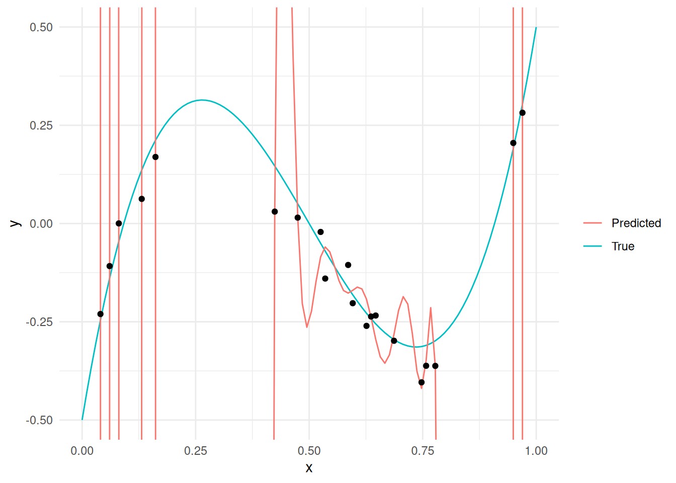
Observations:
- The predictions are perfect at the measured points.
- The predictions are terrible outside the measured points.
The phenomenon we see with the high-degree case above is called overfitting. Overfitting tends to occur when our model is “too flexible”; this excess flexibility allows the model to fit to extraneous patterns, such as measurement noise or data artifacts due to sampling.
So we have a “Goldilocks” problem:
- We need the model to be flexible enough to fit patterns in the data. (Avoid underfitting)
- We need the model to be not too flexible so as not to fit to noise. (Avoid overfitting)
Quantities such as polynomial order that control model flexibility are called hyperparameters; essentially, these are parameters that are not set during the optimization we discussed in e-stat11-models-intro. We might choose to set hyperparameter values based on minimizing the model error.
However, if we try to set the hyperparameters based on the training error, we’re going to make some bad choices. The next task gives us a hint why.
55.3.2 q3 Compute the mse for the 2nd and high-degree polynomial models on df_measurements. Which model has the lower error? Which hyperparameter value (polynomial degree) would you choose, based solely on these numbers?
Hint: We learned how to do this in e-stat11-models-intro.
## [1] 0.03025928## [1] 0.001280951Observations:
fit_overhas lower error ondf_measurements.- Based solely on these results, we would be inclined to choose high-degree polynomial model.
- However, this would be a poor decision, as we have a highly biased measure of model error. We would be better served by studying the error on a validation set.
55.4 A Solution: Validation Data
A solution to the problem above is to reserve a set of validation data to tune the hyperparameters of our model. Note that this requires us to split our data into different sets: training data and validation data. The following code makes that split on df_measurements.
## NOTE: No need to edit this chunk
set.seed(101)

# Select "training" data from our available measurements
df_train <-
  df_measurements %>%
  slice_sample(n = 10)

# Use the remaining data as "validation" data
df_validate <-
  anti_join(
    df_measurements,
    df_train,
    by = "x"
  )

# Visualize the split
df_truth %>%
  ggplot(aes(x, y)) +
  geom_line() +
  geom_point(
    data = df_train %>% mutate(source = "Train"),
    mapping = aes(y = y_meas, color = source)
  ) +
  geom_point(
    data = df_validate %>% mutate(source = "Validate"),
    mapping = aes(y = y_meas, color = source)
  ) +

  scale_color_discrete(name = "Data")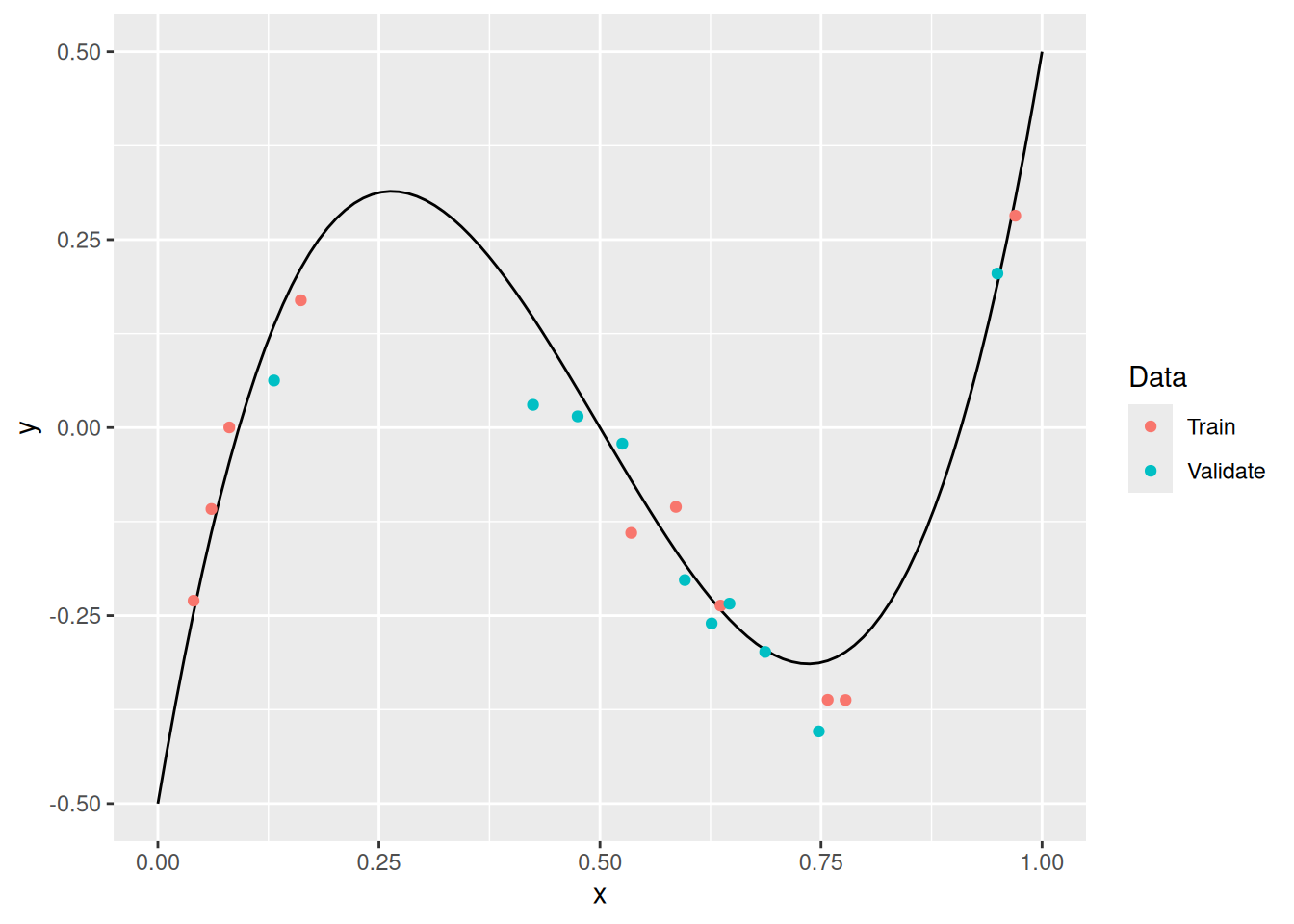
Idea:
- Fit the model on the training data
df_train. - Assess the model on validation data
df_validate. - Use the assessment on validation data to choose the polynomial order.
The following code sweeps through different values of polynomial order, fits a polynomial, and computes the associated error on both the Train and Validate sets.
## NOTE: No need to change this code
df_sweep <-
  map_dfr(
    seq(1, 9, by = 1),
    function(order) {
      # Fit a temporary model
      fit_tmp <-
        lm(
          data = df_train,
          formula = y_meas ~ poly(x, order)
        )

      # Compute error on the Train and Validate sets
      tibble(
        error_Train = mse(fit_tmp, df_train),
        error_Validate = mse(fit_tmp, df_validate),
        order = order
      )
    }
  ) %>%
  pivot_longer(
    names_to = c(".value", "source"),
    names_sep = "_",
    cols = matches("error")
  )
In the next task, you will compare the resulting error metrics.
55.4.1 q4 Inspect the results of the degree sweep, and answer the questions below.
## NOTE: No need to edit; inspect and write your observations
df_sweep %>%
  ggplot(aes(order, error, color = source)) +
  geom_line() +

  scale_y_log10() +
  scale_x_continuous(breaks = seq(1, 10, by = 1)) +
  scale_color_discrete(name = "Method") +
  coord_cartesian(ylim = c(1e-3, 1)) +
  theme(legend.position = "bottom") +
  labs(
    x = "Polynomial Order",
    y = "Mean Squared Error"
  )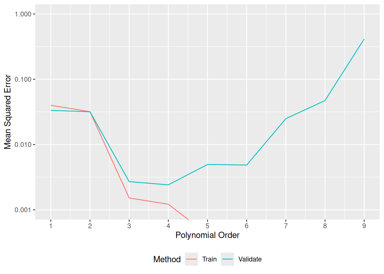
Observations
- Training error is minimized at polynomial order 8, or possibly higher.
- Validation error is minimized at polynomial order 3.
- Selecting the polynomial order via the validation error leads to the correct choice.
55.5 Intermediate Summary
We’ve seen a few ideas:
- A model that is not flexible enough will tend to underfit a dataset.
- A model that is too flexible will tend to overfit a dataset.
- The training error is an optimistic measure of accuracy, it is not an appropriate metric for setting hyperparameter values.
- To set hyperparameter values, we are better off “holding out” a validation set from our data, and using the validation error to make model decisions.
55.6 More Challenging Case: Modeling Diamond Prices
Above we made our model more flexible by changing the polynomial order. For instance, a 2nd-order polynomial model would be
\[\hat{y}_2 = \beta_0 + \beta_1 x + \beta_2 x^2 + \epsilon,\]
while a 5th-order polynomial model would be
\[\hat{y}_5 = \beta_0 + \beta_1 x + \beta_2 x^2+ \beta_3 x^3+ \beta_4 x^4 + \beta_5 x^5 + \epsilon.\]
In effect, we are adding another predictor of the form \(\beta_i x^i\) every time we increase the polynomial order. Increasing polynomial order is just one way we increase model flexibility; another way is to add additional variables to the model.
For instance, in the diamonds dataset we have a number of variables that we could use as predictors:
## [1] "carat"   "cut"     "color"   "clarity" "depth"   "table"   "x"
## [8] "y"       "z"
Let’s put the train-validation idea to work! Below I set up training and validation sets of the diamonds data, and train a very silly model that blindly uses all the variables available as predictors. The challenge: Can you beat this model?
## NOTE: No need to edit this setup
# Create a test-validate split
set.seed(101)
diamonds_randomized <-
  diamonds %>%
  slice(sample(dim(diamonds)[1]))

diamonds_train <-
  diamonds_randomized %>%
  slice(1:10000)

diamonds_validate <-
  diamonds_randomized %>%
  slice(10001:20000)

# Try to beat this naive model that uses all variables!
fit_full <-
  lm(
    data = diamonds_train,
    formula = price ~ . # The `.` notation here means "use all variables"
  )
55.6.1 q5 Build your own model!
Choose which predictors to include by modifying the formula argument below. Use the validation data to help guide your choice. Answer the questions below.
Hint: We’ve done EDA on diamonds before. Use your knowledge from that past EDA to choose variables you think will be informative for predicting the price.
## NOTE: This is just one possible model!
fit_q5 <-
  lm(
    data = diamonds_train,
    formula = price ~ carat + cut + color + clarity
  )

# Compare the two models on the validation set
mse(fit_q5, diamonds_validate)
## [1] 1306804## [1] 1568726Observations:
caratby itself does a decent job predictingprice.- Based on EDA we’ve done before, it appears that
caratis the major decider in diamond price.
- Based on EDA we’ve done before, it appears that
cut,color, andclarityhelp, but do not have the same predictive power (by themselves) ascarat.- Based on EDA we’ve done before, we know that
cut,color, andclarityare important forprice, but not quite as important ascarat.
- Based on EDA we’ve done before, we know that
x,y, andzalone have predictive power similar tocaratalone. They probably correlate well with the weight, as they measure the dimensions of the diamond.x,y, andztogether have very poor predictive powerdepthandtabledo not have the same predictive power ascarat.- The best combination of predictors I found was
carat + cut + color + clarity.
Aside: The process of choosing predictors—sometimes called features—is called feature selection.
One last thing: Note above that I first randomized the diamonds before selecting training and validation data. This is really important! Let’s see what happens if we don’t randomize the data before splitting:
55.6.2 q6 Visualize a histogram for the prices of diamonds_train_bad and diamonds_validate_bad. Answer the questions below.
## NOTE: No need to edit this part
diamonds_train_bad <-
  diamonds %>%
  slice(1:10000)

diamonds_validate_bad <-
  diamonds %>%
  slice(10001:20000)

## TODO: Visualize a histogram of prices for both `bad` sets.
bind_rows(
  diamonds_train_bad %>% mutate(source = "Train"),
  diamonds_validate_bad %>% mutate(source = "Validate")
) %>%
  ggplot(aes(price)) +
  geom_histogram(bins = 100) +

  facet_grid(source ~ .)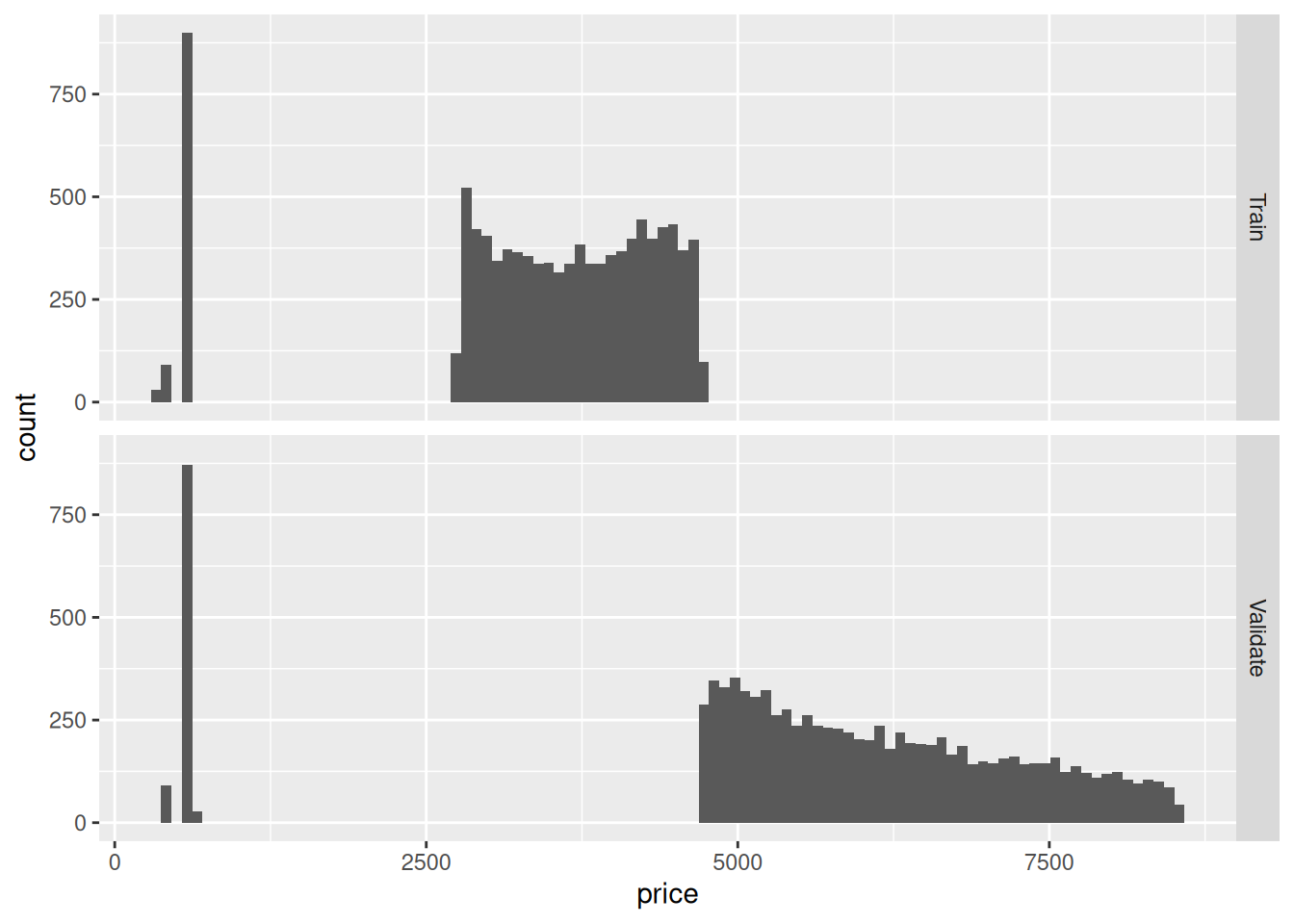
Observations:
diamonds_test_badanddiamonds_validate_badhave very little overlap! It seems thediamondsdatset has some ordering alongprice, which greatly affects our split.- If we were to train and then validate, we would be training on lower-price diamonds and predicting on higher-price diamonds. This might actually be appropriate if we’re trying to extrapolate from low to high. But if we are trying to get a representative estimate of error for training, this would be an inappropriate split.