37 Data: Reading Excel Sheets
Purpose: The Tidyverse is built to work with tidy data. Unfortunately, most data in the wild are not tidy. The good news is that we have a lot of tools for wrangling data into tidy form. The bad news is that “every untidy dataset is untidy in its own way.” I can’t show you you every crazy way people decide to store their data. But I can walk you through a worked example to show some common techniques.
In this case study, I’ll take you through the process of wrangling a messy Excel spreadsheet into machine-readable form. You will both learn some general tools for wrangling data, and you can keep this notebook as a recipe for future messy datasets of similar form.
Reading: (None)
## ── Attaching core tidyverse packages ──────────────────────── tidyverse 2.0.0 ──
## ✔ dplyr     1.1.4     ✔ readr     2.1.5
## ✔ forcats   1.0.0     ✔ stringr   1.5.1
## ✔ ggplot2   3.5.2     ✔ tibble    3.2.1
## ✔ lubridate 1.9.4     ✔ tidyr     1.3.1
## ✔ purrr     1.0.4
## ── Conflicts ────────────────────────────────────────── tidyverse_conflicts() ──
## ✖ dplyr::filter() masks stats::filter()
## ✖ dplyr::lag()    masks stats::lag()
## ℹ Use the conflicted package (<http://conflicted.r-lib.org/>) to force all conflicts to become errorslibrary(readxl) # For reading Excel sheets
library(httr) # For downloading files
## Use my tidy-exercises copy of UNDOC data for stability
url_undoc <- "https://github.com/zdelrosario/tidy-exercises/blob/master/2019/2019-12-10-news-plots/GSH2013_Homicide_count_and_rate.xlsx?raw=true"
filename <- "./data/undoc.xlsx"I keep a copy of the example data in a personal repo; download a local copy.
37.1 Wrangling Basics
37.1.1 q1 Run the following code and pay attention to the column names. Open the downloaded Excel sheet and compare. Why are the column names so weird?
## New names:
## • `` -> `...2`
## • `` -> `...3`
## • `` -> `...4`
## • `` -> `...5`
## • `` -> `...6`
## • `` -> `...7`
## • `` -> `...8`
## • `` -> `...9`
## • `` -> `...10`
## • `` -> `...11`
## • `` -> `...12`
## • `` -> `...13`
## • `` -> `...14`
## • `` -> `...15`
## • `` -> `...16`
## • `` -> `...17`
## • `` -> `...18`
## • `` -> `...19`## Rows: 447
## Columns: 19
## $ `Intentional homicide count and rate per 100,000 population, by country/territory (2000-2012)` <chr> …
## $ ...2 <chr> …
## $ ...3 <chr> …
## $ ...4 <chr> …
## $ ...5 <chr> …
## $ ...6 <chr> …
## $ ...7 <chr> …
## $ ...8 <dbl> …
## $ ...9 <dbl> …
## $ ...10 <dbl> …
## $ ...11 <dbl> …
## $ ...12 <dbl> …
## $ ...13 <dbl> …
## $ ...14 <dbl> …
## $ ...15 <dbl> …
## $ ...16 <chr> …
## $ ...17 <chr> …
## $ ...18 <chr> …
## $ ...19 <chr> …Observations:
- The top row is filled with expository text. The actual column names are several rows down.
Most read_ functions have a skip argument you can use to skip over the first few lines. Use this argument in the next task to deal with the top of the Excel sheet.
37.1.2 q2 Read the Excel sheet.
Open the target Excel sheet (located at ./data/undoc.xlsx) and find which line (row) at which the year column headers are located. Use the skip keyword to start your read at that line.
## New names:
## • `` -> `...1`
## • `` -> `...2`
## • `` -> `...3`
## • `` -> `...4`
## • `` -> `...5`
## • `` -> `...6`## Rows: 444
## Columns: 19
## $ ...1 <chr> "Africa", NA, NA, NA, NA, NA, NA, NA, NA, NA, NA, NA, NA, NA, N…
## $ ...2 <chr> "Eastern Africa", NA, NA, NA, NA, NA, NA, NA, NA, NA, NA, NA, N…
## $ ...3 <chr> "Burundi", NA, "Comoros", NA, "Djibouti", NA, "Eritrea", NA, "E…
## $ ...4 <chr> "PH", NA, "PH", NA, "PH", NA, "PH", NA, "PH", NA, "CJ", NA, "PH…
## $ ...5 <chr> "WHO", NA, "WHO", NA, "WHO", NA, "WHO", NA, "WHO", NA, "CTS", N…
## $ ...6 <chr> "Rate", "Count", "Rate", "Count", "Rate", "Count", "Rate", "Cou…
## $ `2000` <dbl> NA, NA, NA, NA, NA, NA, NA, NA, NA, NA, NA, NA, NA, NA, 6.2, 70…
## $ `2001` <dbl> NA, NA, NA, NA, NA, NA, NA, NA, NA, NA, NA, NA, NA, NA, 7.7, 90…
## $ `2002` <dbl> NA, NA, NA, NA, NA, NA, NA, NA, NA, NA, NA, NA, NA, NA, 4.8, 56…
## $ `2003` <dbl> NA, NA, NA, NA, NA, NA, NA, NA, NA, NA, NA, NA, NA, NA, 2.5, 30…
## $ `2004` <dbl> NA, NA, NA, NA, NA, NA, NA, NA, NA, NA, 4.0, 1395.0, NA, NA, 3.…
## $ `2005` <dbl> NA, NA, NA, NA, NA, NA, NA, NA, NA, NA, 3.5, 1260.0, NA, NA, 1.…
## $ `2006` <dbl> NA, NA, NA, NA, NA, NA, NA, NA, NA, NA, 3.5, 1286.0, NA, NA, 6.…
## $ `2007` <dbl> NA, NA, NA, NA, NA, NA, NA, NA, NA, NA, 3.4, 1281.0, NA, NA, 5.…
## $ `2008` <dbl> NA, NA, NA, NA, NA, NA, NA, NA, NA, NA, 3.6, 1413.0, NA, NA, 5.…
## $ `2009` <chr> NA, NA, NA, NA, NA, NA, NA, NA, NA, NA, "5.6", "2218", NA, NA, …
## $ `2010` <chr> NA, NA, NA, NA, NA, NA, NA, NA, NA, NA, "5.5", "2239", NA, NA, …
## $ `2011` <chr> NA, NA, NA, NA, NA, NA, NA, NA, NA, NA, "6.3", "2641", NA, NA, …
## $ `2012` <chr> "8", "790", "10", "72", "10.1", "87", "7.1", "437", "12", "1104…Use the following test to check your work.
## NOTE: No need to change this
assertthat::assert_that(setequal(
              (df_q2 %>% names() %>% .[7:19]),
              as.character(seq(2000, 2012))
            ))
## [1] TRUE## [1] "Nice!"Let’s take stock of where we are:
## # A tibble: 6 × 19
##   ...1   ...2  ...3  ...4  ...5  ...6  `2000` `2001` `2002` `2003` `2004` `2005`
##   <chr>  <chr> <chr> <chr> <chr> <chr>  <dbl>  <dbl>  <dbl>  <dbl>  <dbl>  <dbl>
## 1 Africa East… Buru… PH    WHO   Rate      NA     NA     NA     NA     NA     NA
## 2 <NA>   <NA>  <NA>  <NA>  <NA>  Count     NA     NA     NA     NA     NA     NA
## 3 <NA>   <NA>  Como… PH    WHO   Rate      NA     NA     NA     NA     NA     NA
## 4 <NA>   <NA>  <NA>  <NA>  <NA>  Count     NA     NA     NA     NA     NA     NA
## 5 <NA>   <NA>  Djib… PH    WHO   Rate      NA     NA     NA     NA     NA     NA
## 6 <NA>   <NA>  <NA>  <NA>  <NA>  Count     NA     NA     NA     NA     NA     NA
## # ℹ 7 more variables: `2006` <dbl>, `2007` <dbl>, `2008` <dbl>, `2009` <chr>,
## #   `2010` <chr>, `2011` <chr>, `2012` <chr>
We still have problems:
- The first few columns don’t have sensible names. The
col_namesargument allows us to set manual names at the read phase. - Some of the columns are of the wrong type; for instance
2012is achrvector. We can use thecol_typesargument to set manual column types.
37.1.3 q3 Change the column names and types.
Use the provided names in col_names_undoc with the col_names argument to set manual column names. Use the col_types argument to set all years to "numeric", and the rest to "text".
Hint 1: Since you’re providing manual col_names, you will have to adjust your skip value!
Hint 2: You can use a named vector for col_types to help keep type of which type is assigned to which variable, for instance c("variable" = "type").
## NOTE: Use these column names
col_names_undoc <-
  c(
    "region",
    "sub_region",
    "territory",
    "source",
    "org",
    "indicator",
    "2000",
    "2001",
    "2002",
    "2003",
    "2004",
    "2005",
    "2006",
    "2007",
    "2008",
    "2009",
    "2010",
    "2011",
    "2012"
  )

## TASK: Use the arguments `skip`, `col_names`, and `col_types`
df_q3 <- read_excel(
  filename,
  sheet = 1,
  skip = 7,
  col_names = col_names_undoc,
  col_types = c(
    "region"     = "text",
    "sub_region" = "text",
    "territory"  = "text",
    "source"     = "text",
    "org"        = "text",
    "indicator"  = "text",
    "2000" = "numeric",
    "2001" = "numeric",
    "2002" = "numeric",
    "2003" = "numeric",
    "2004" = "numeric",
    "2005" = "numeric",
    "2006" = "numeric",
    "2007" = "numeric",
    "2008" = "numeric",
    "2009" = "numeric",
    "2010" = "numeric",
    "2011" = "numeric",
    "2012" = "numeric"
  )
)
## Warning: Expecting numeric in P315 / R315C16: got '2366*'## Warning: Expecting numeric in Q315 / R315C17: got '1923*'## Warning: Expecting numeric in R315 / R315C18: got '1866*'## Warning: Expecting numeric in S381 / R381C19: got 'x'## Warning: Expecting numeric in S431 / R431C19: got 'x'## Warning: Expecting numeric in S433 / R433C19: got 'x'## Warning: Expecting numeric in S435 / R435C19: got 'x'## Warning: Expecting numeric in S439 / R439C19: got 'x'## Warning: Expecting numeric in S445 / R445C19: got 'x'Use the following test to check your work.
## NOTE: No need to change this
assertthat::assert_that(setequal(
              (df_q3 %>% names()),
              col_names_undoc
            ))
## [1] TRUE## [1] TRUE## [1] "Great!"37.2 Danger Zone
Now let’s take a look at the head of the data:
## # A tibble: 6 × 19
##   region sub_region territory source org   indicator `2000` `2001` `2002` `2003`
##   <chr>  <chr>      <chr>     <chr>  <chr> <chr>      <dbl>  <dbl>  <dbl>  <dbl>
## 1 Africa Eastern A… Burundi   PH     WHO   Rate          NA     NA     NA     NA
## 2 <NA>   <NA>       <NA>      <NA>   <NA>  Count         NA     NA     NA     NA
## 3 <NA>   <NA>       Comoros   PH     WHO   Rate          NA     NA     NA     NA
## 4 <NA>   <NA>       <NA>      <NA>   <NA>  Count         NA     NA     NA     NA
## 5 <NA>   <NA>       Djibouti  PH     WHO   Rate          NA     NA     NA     NA
## 6 <NA>   <NA>       <NA>      <NA>   <NA>  Count         NA     NA     NA     NA
## # ℹ 9 more variables: `2004` <dbl>, `2005` <dbl>, `2006` <dbl>, `2007` <dbl>,
## #   `2008` <dbl>, `2009` <dbl>, `2010` <dbl>, `2011` <dbl>, `2012` <dbl>
Irritatingly, many of the cell values are left implicit; as humans reading these data, we can tell that the entries in region under Africa also have the value Africa. However, the computer can’t tell this! We need to make these values explicit by filling them in.
To that end, I’m going to guide you through some slightly advanced Tidyverse code to lag-fill the missing values. To that end, I’ll define and demonstrate two helper functions:
First, the following function counts the number of rows with NA entries in a chosen set of columns:
## Helper function to count num rows w/ NA in vars_lagged
rowAny <- function(x) rowSums(x) > 0
countna <- function(df, vars_lagged) {
  df %>%
    filter(rowAny(across(vars_lagged, is.na))) %>%
    dim %>%
    .[[1]]
}

countna(df_q3, c("region"))
## Warning: There was 1 warning in `filter()`.
## ℹ In argument: `rowAny(across(vars_lagged, is.na))`.
## Caused by warning:
## ! Using an external vector in selections was deprecated in tidyselect 1.1.0.
## ℹ Please use `all_of()` or `any_of()` instead.
## # Was:
## data %>% select(vars_lagged)
##
## # Now:
## data %>% select(all_of(vars_lagged))
##
## See <https://tidyselect.r-lib.org/reference/faq-external-vector.html>.## [1] 435Ideally we want this count to be zero. To fill-in values, we will use the following function to do one round of lag-filling:
lagfill <- function(df, vars_lagged) {
  df %>%
    mutate(across(
      vars_lagged,
      function(var) {
        if_else(
          is.na(var) & !is.na(lag(var)),
          lag(var),
          var
        )
      }
    ))
}

df_tmp <-
  df_q3 %>%
  lagfill(c("region"))

countna(df_tmp, c("region"))
## [1] 429We can see that lagfill has filled the Africa value in row 2, as well as a number of other rows as evidenced by the reduced value returned by countna.
What we’ll do is continually run lagfill until we reduce countna to zero. We could do this by repeatedly running the function manually, but that would be silly. Instead, we’ll run a while loop to automatically run the function until countna reaches zero.
37.2.1 q4 I have already provided the while loop below; fill in vars_lagged with the names of the columns where cell values are implicit.
Hint: Think about which columns have implicit values, and which truly have missing values.
## Choose variables to lag-fill
vars_lagged <- c("region", "sub_region", "territory", "source", "org")

## NOTE: No need to edit this
## Trim head and notes
df_q4 <-
  df_q3 %>%
  slice(-(n()-5:-n()))

## Repeatedly lag-fill until NA's are gone
while (countna(df_q4, vars_lagged) > 0) {
  df_q4 <-
    df_q4 %>%
    lagfill(vars_lagged)
}
And we’re done! All of the particularly tricky wrangling is now done. You could now use pivoting to tidy the data into long form.
Purpose: The sampling distribution is a key object in statistics—it helps us understand how good our estimates are. However, following the definition is an impractical way to compute a sampling distribution. In this exercise we’ll learn about a practical recipe for estimating a sampling distribution—bootstrap resampling.
Reading: (None, this is the reading)
Topics: Resampling and inference
## ── Attaching core tidyverse packages ──────────────────────── tidyverse 2.0.0 ──
## ✔ dplyr     1.1.4     ✔ readr     2.1.5
## ✔ forcats   1.0.0     ✔ stringr   1.5.1
## ✔ ggplot2   3.5.2     ✔ tibble    3.2.1
## ✔ lubridate 1.9.4     ✔ tidyr     1.3.1
## ✔ purrr     1.0.4
## ── Conflicts ────────────────────────────────────────── tidyverse_conflicts() ──
## ✖ dplyr::filter() masks stats::filter()
## ✖ dplyr::lag()    masks stats::lag()
## ℹ Use the conflicted package (<http://conflicted.r-lib.org/>) to force all conflicts to become errors37.3 The Core Idea: Resampling with Replacement
In the previous exercise (e-stat04-population) we learned about the difference between a population and a sample. We also talked about sampling distributions—a sampling distribution is a theoretical distribution where we repeatedly gather a sample (of fixed size \(n\)) from the population, and compute the same summary statistic each time. The distribution of the summary statistic is the sampling distribution.
However, this theoretical recipe is not a practical idea: It would be silly to gather many small samples and analyze them separately. If we’ve worked hard to gather a large dataset, we should just analyze it all together. To overcome this practical hurdle, we’ll use the idea of resampling—this is based on a key assumption, that our sample is representative of our population.
Here’s a sample from a normal distribution (population). For ease of comparison, we draw the normal distribution as a solid curve.
## NOTE: No need to edit this setup
set.seed(101) # Set a seed for reproducibility

mu <- 0
sd <- 1
n <- 50

df_data_norm <- tibble(x = rnorm(n, mean = mu, sd = sd))

df_data_norm %>%
  ggplot(aes(x)) +
  geom_histogram(aes(y = after_stat(..density..))) +
  geom_line(
    aes(y = d),
    data = tibble(x = seq(-2.5, +1.5, length.out = 500)) %>%
      mutate(d = dnorm(x, mean = mu, sd = sd)),
    color = "salmon"
  )
## `stat_bin()` using `bins = 30`. Pick better value with `binwidth`.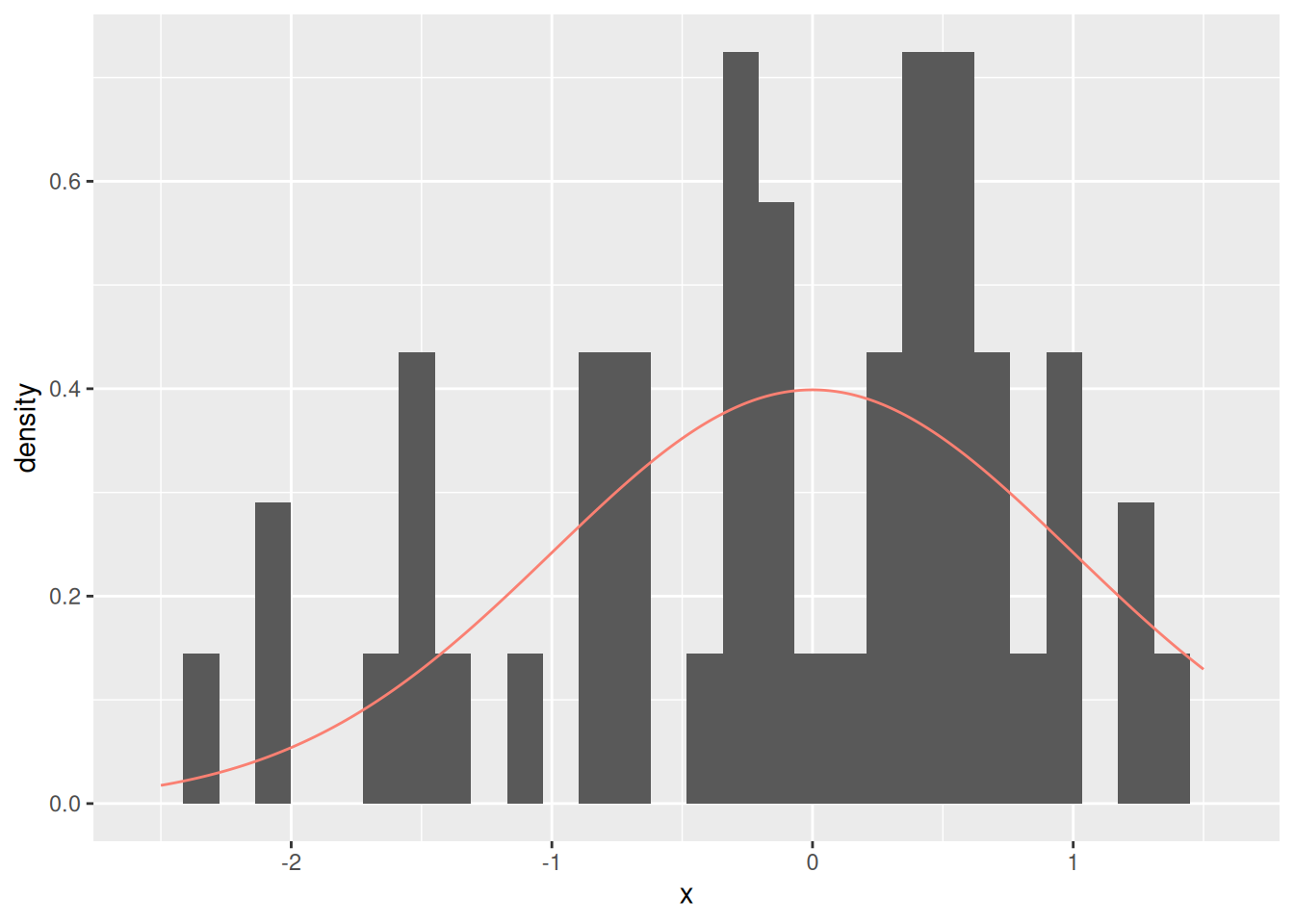
The sample (histogram) does not look identical to the population (solid curve). But it can’t, because we don’t have all the observations in the population. The key assumption we make in statistical inference is that the sample “looks like” the population. In technical terms, such a sample is representative of a chosen population.
The way we use this assumption is to treat our sample as though it were the population. This is subtle though. If we resample our entire sample, we end up with exactly the same sample. That’s not helpful!
## NOTE: Do not edit this code
# This is the **WRONG** way to do resampling
df_data_norm %>%
  # Resample *without* replacement
  pull(x) %>%
  sample(., size = n, replace = FALSE) %>%
  tibble(x = ., source = "Resampled") %>%
  # Visualize against the original sample
  bind_rows(., df_data_norm %>% mutate(source = "Original")) %>%
  ggplot(aes(x)) +
  geom_freqpoly(aes(color = source, linetype = source), bins = 15)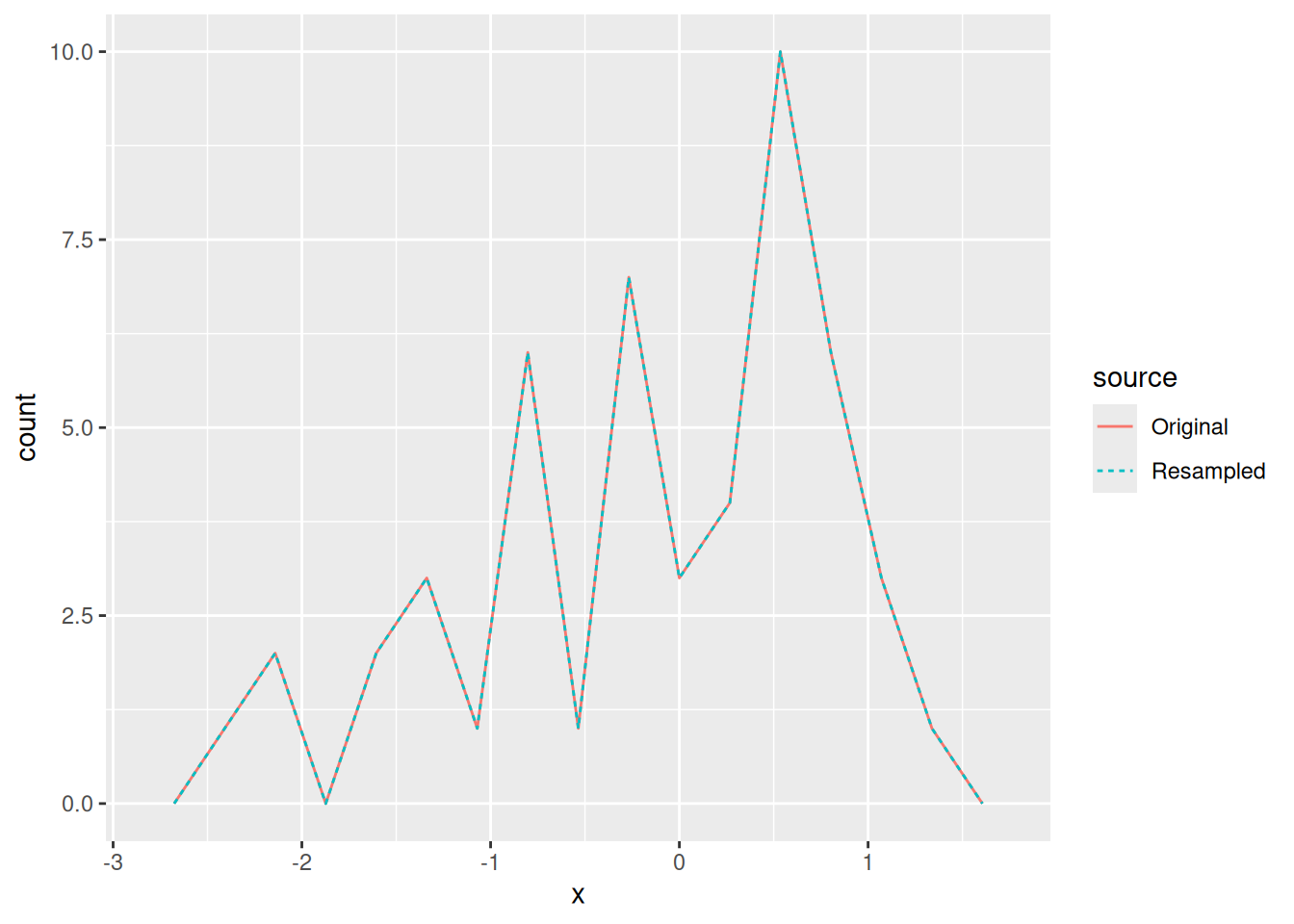
Note that the Resampled set looks exactly like the Original sample. This is not what we want. Instead, we have to resample with replacement.
## NOTE: Do not edit this code
# This is the **RIGHT** way to do resampling
df_data_norm %>%
  # Resample *with* replacement
  pull(x) %>%
  sample(., size = n, replace = TRUE) %>%
  tibble(x = ., source = "Resampled") %>%
  # Visualize against the original sample
  bind_rows(., df_data_norm %>% mutate(source = "Original")) %>%
  ggplot(aes(x)) +
  geom_freqpoly(aes(color = source, linetype = source), bins = 15)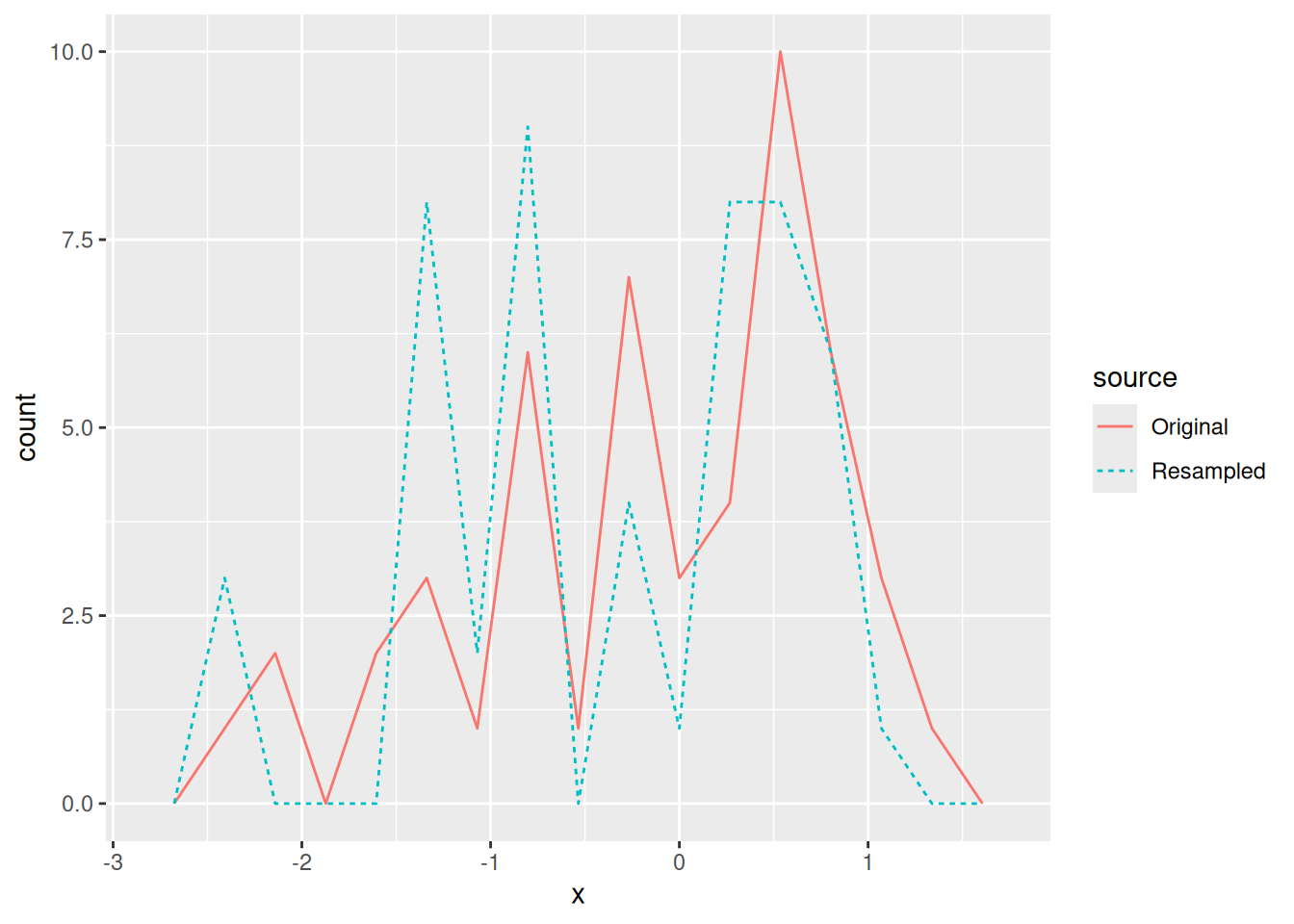
Once we have resampled the sample, we can compute any statistics we care about:
## NOTE: Do not edit this code
# This is the **RIGHT** way to do resampling
df_data_norm %>%
  # Resample *with* replacement
  pull(x) %>%
  sample(., size = n, replace = TRUE) %>%
  tibble(x = ., source = "Resampled") %>%
  # Compute statistics we care about
  bind_rows(., df_data_norm %>% mutate(source = "Original")) %>%
  group_by(source) %>%
  summarize(
    sample_mean = mean(x),
    sample_sd = sd(x)
  )
## # A tibble: 2 × 3
## source sample_mean sample_sd
## <chr> <dbl> <dbl>
## 1 Original -0.124 0.932
## 2 Resampled 0.103 0.763This is the core idea of resampling. But to simulate a sampling distribution, we need to do this many times.
37.3.1 Efficient resampling
The code we just saw is computationally wasteful, since it stores the same data in many copies. So, programmers have written efficient packages to support resampling methods. We will use the rsample package for resampling in this class. The bootstraps() function resamples with replacement a desired number of times.
Note: Bootstrap resampling is just one of many kinds of resampling methods. It’s called “bootstrapping” because we’re “pulling ourselves up by our own bootstraps”, in the sense that we’re only using the sample we have at hand.
## # Bootstrap sampling
## # A tibble: 1,000 × 2
## splits id
## <list> <chr>
## 1 <split [50/16]> Bootstrap0001
## 2 <split [50/19]> Bootstrap0002
## 3 <split [50/16]> Bootstrap0003
## 4 <split [50/21]> Bootstrap0004
## 5 <split [50/18]> Bootstrap0005
## 6 <split [50/16]> Bootstrap0006
## 7 <split [50/15]> Bootstrap0007
## 8 <split [50/17]> Bootstrap0008
## 9 <split [50/22]> Bootstrap0009
## 10 <split [50/23]> Bootstrap0010
## # ℹ 990 more rowsThis looks weird; we have 1000 rows, corresponding to times = 1000. The splits column is where the programming magic happens: Rather than storing a copy of the original data, a split is a list of observations to use in a resample. To take advantage of bootstraps(), we have to use the anaysis() function on the splits column. Here’s an example of accessing a single resample:
## NOTE: No need to edit
df_data_norm %>%
bootstraps(., times = 1) %>%
# Pull out a single `splits` object
pull(splits) %>%
.[[1]] %>%
# Use analysis() to turn the split into a usable dataset
analysis()## # A tibble: 50 × 1
## x
## <dbl>
## 1 -1.46
## 2 -0.223
## 3 0.758
## 4 1.17
## 5 0.920
## 6 0.279
## 7 0.569
## 8 -0.223
## 9 0.448
## 10 0.403
## # ℹ 40 more rowsThe following code uses bootstraps() and analysis() to show the first 9 resamplings.
## NOTE: No need to edit this setup
df_resample_norm <-
bootstraps(df_data_norm, times = 1000) %>%
mutate(df = map(splits, ~ analysis(.x)))
# Visualize the first 9 of the resamples
df_resample_norm %>%
slice(1:9) %>%
unnest(df) %>%
ggplot(aes(x)) +
geom_histogram() +
facet_wrap(~ id)## `stat_bin()` using `bins = 30`. Pick better value with `binwidth`.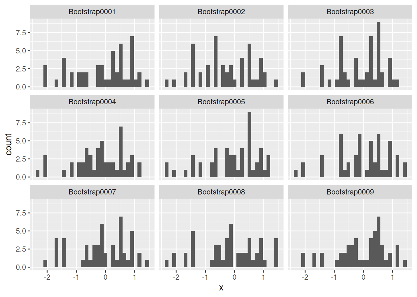
In the example above, I set times = 1000 but show only the first nine. Generally, a larger value of times is better, but a good rule of thumb is to do at least 1000 resamples.
Side Notes:
- The
bootstraps()function comes from thersamplepackage, which implements many different resampling strategies (beyond the bootstrap). - The
analysis()function also comes fromrsample; this is a special function we need to call when working with a resampling of the data [1]. - We saw the
map()function ine-data10-map; usingmap()above is necessary in part because we need to callanalysis(). Sinceanalysis()is not vectorized, we need the map to use this function on every split insplits.
37.3.2 Using resampling
Working with bootstraps() can be a little finicky. Here’s some example code you can adapt for future use.
Fundamentally, this code is resampling the data with replacement, and carrying out an analysis on each (resampled) dataset using a function we provide.
## NOTE: No need to edit this example
# Start with our dataset
df_demo <-
df_data_norm %>%
# Create the bootstrap resamplings
bootstraps(., times = 1000) %>%
# Finicky code: Compute an estimate for each resampling (`splits` column)
mutate(
# The `map_*` family of functions iterates a provided function over a column
sample_mean = map_dbl(
# Chosen column
splits,
# Function we provide (defined inline)
function(split_df) {
# First, we use `analysis()` to translate the split into usable data
split_df %>%
analysis() %>%
# Then, we carry out whatever analysis we want
summarize(sample_mean = mean(x)) %>%
# One last wrangling step
pull(sample_mean)
}
)
)
df_demo ## # Bootstrap sampling
## # A tibble: 1,000 × 3
## splits id sample_mean
## <list> <chr> <dbl>
## 1 <split [50/18]> Bootstrap0001 -0.118
## 2 <split [50/22]> Bootstrap0002 -0.301
## 3 <split [50/19]> Bootstrap0003 -0.0764
## 4 <split [50/17]> Bootstrap0004 -0.180
## 5 <split [50/20]> Bootstrap0005 0.0279
## 6 <split [50/19]> Bootstrap0006 -0.195
## 7 <split [50/17]> Bootstrap0007 -0.222
## 8 <split [50/17]> Bootstrap0008 -0.188
## 9 <split [50/22]> Bootstrap0009 0.0463
## 10 <split [50/18]> Bootstrap0010 -0.184
## # ℹ 990 more rows37.3.3 q1 Modify the code
Copy and modify the previous code to estimate a sampling distribution for the standard deviation. Provide this as a column sample_sd.
df_q1 <-
df_data_norm %>%
bootstraps(., times = 1000) %>%
mutate(
sample_sd = map_dbl(
splits,
function(split_df) {
split_df %>%
analysis() %>%
summarize(sample_sd = sd(x)) %>%
pull(sample_sd)
}
)
)
df_q1## # Bootstrap sampling
## # A tibble: 1,000 × 3
## splits id sample_sd
## <list> <chr> <dbl>
## 1 <split [50/17]> Bootstrap0001 0.762
## 2 <split [50/16]> Bootstrap0002 0.990
## 3 <split [50/15]> Bootstrap0003 0.919
## 4 <split [50/20]> Bootstrap0004 0.985
## 5 <split [50/22]> Bootstrap0005 0.898
## 6 <split [50/17]> Bootstrap0006 0.909
## 7 <split [50/17]> Bootstrap0007 0.916
## 8 <split [50/21]> Bootstrap0008 1.08
## 9 <split [50/17]> Bootstrap0009 0.968
## 10 <split [50/17]> Bootstrap0010 1.10
## # ℹ 990 more rowsThe following test will verify that your df_q1 is correct:
## NOTE: No need to change this!
assertthat::assert_that(
    df_q1 %>%
      mutate(
        test_sd = map_dbl(splits, ~analysis(.) %>% summarize(s = sd(x)) %>% pull(s)),
        test = test_sd == sample_sd
      ) %>%
      pull(test) %>%
      all()
)
## [1] TRUE## [1] "Great job!"The following code will visualize your results.
## `stat_bin()` using `bins = 30`. Pick better value with `binwidth`.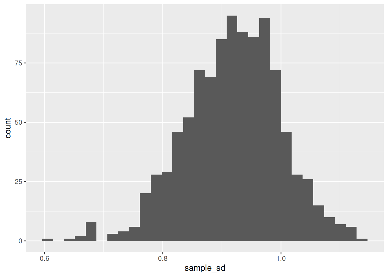
This plot gives us an (approximate) sampling distribution for the standard deviation. A reasonable next step would be to compute the standard error.
37.3.4 q2 Compute the standard error
Compute the standard error for the mean by completing the code below.
Hint: We defined the standard error in the previous stat exercise (e-stat04).
## TASK: Compute the standard error
df_q2 <-
  df_data_norm %>%
  bootstraps(., times = 1000) %>%
  mutate(
    sample_mean = map_dbl(
      splits,
      function(split_df) {
        split_df %>%
          analysis() %>%
          summarize(sample_mean = mean(x)) %>%
          pull(sample_mean)
      }
    )
  ) %>%
  summarize(se = sd(sample_mean))

df_q2
## # A tibble: 1 × 1
## se
## <dbl>
## 1 0.134The following test will verify that your df_q2 is correct:
## NOTE: No need to change this!
assertthat::assert_that(
    (df_q2 %>% pull(se)) > 0.1,
    msg = "Take a closer look at the definition of the standard error. We only divide by sqrt(n) when using the standard deviation of the *population* (not the standard deviation of the *samping distribution*)."
)
## [1] TRUE## [1] "Great job!"We can use a sampling distribution to build a “reasonable interval” for the population value we’re trying to estimate. We can do this by taking quantiles of the distribution.
37.3.5 q3 Quantiles of the sampling distribution
Compute the lower and upper quantiles of the sampling distribution for the mean, such that 0.99 of the distribution is contained within the endpoints, and an equal amount of the distribution lands on either side outside the endpoints.
Hint: You should use the alpha provided below, but you need to select half of alpha from the left tail, and half from the right tail.
## TASK: Compute the lower and upper quantiles of the sampling distribution
alpha <- 0.01

df_q3 <-
  df_demo %>%
  summarize(
# task_begin
    # mean_lo = ?,
    # mean_up = ?,
# task_end
    mean_lo = quantile(sample_mean, alpha / 2),
    mean_up = quantile(sample_mean, 1 - alpha / 2),
  )
The following will visualize your results against the sampling distribution:
## NOTE: Do not edit this code
df_demo %>%
  ggplot(aes(sample_mean)) +
  geom_histogram() +
  geom_vline(
    data = df_q3,
    mapping = aes(xintercept = mean_lo)
  ) +
  geom_vline(
    data = df_q3,
    mapping = aes(xintercept = mean_up)
  )
## `stat_bin()` using `bins = 30`. Pick better value with `binwidth`.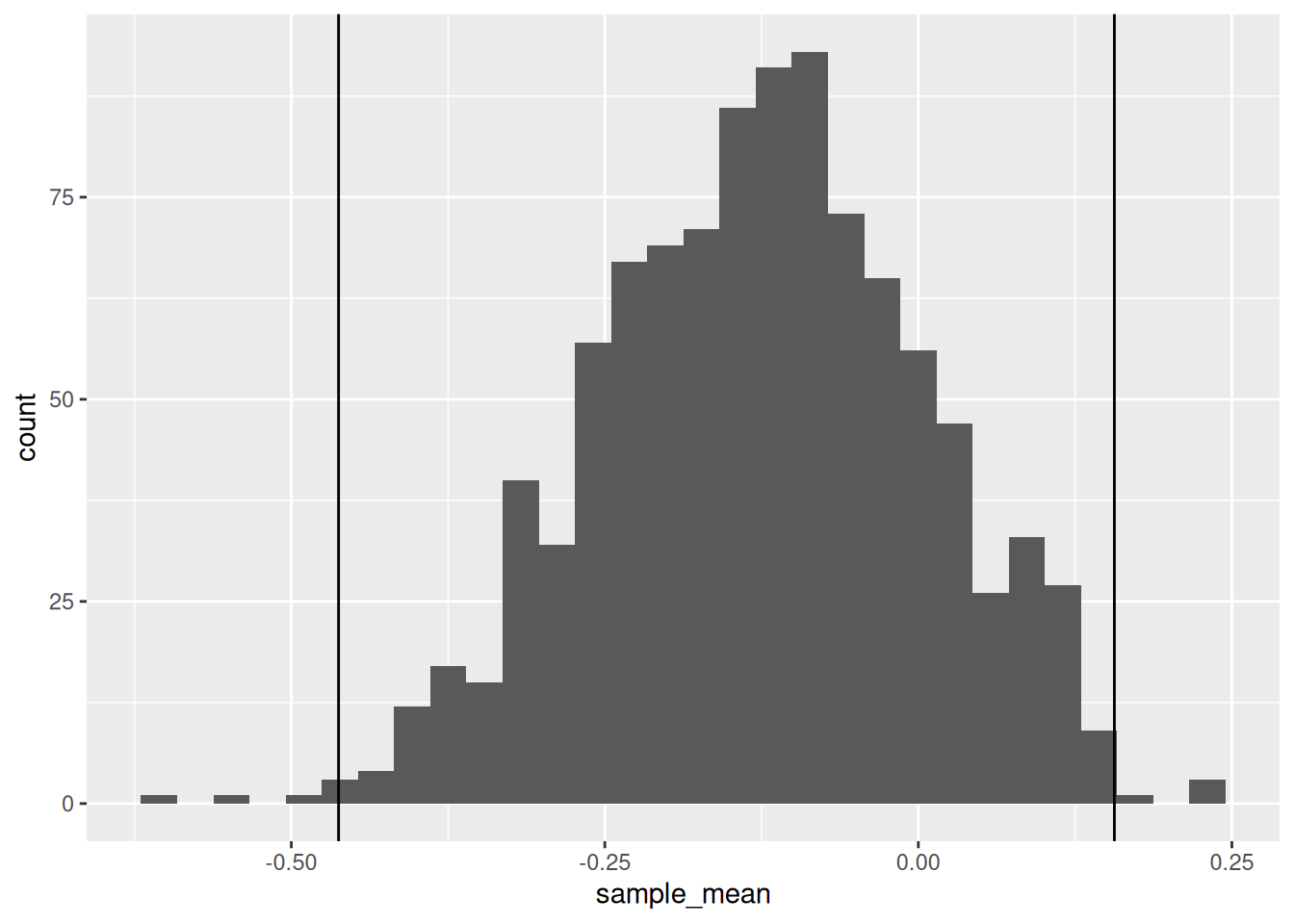
The following test will verify that your df_q2 is correct:
## NOTE: No need to change this!
assertthat::assert_that(
    abs(
      df_q3 %>% pull(mean_lo) %>% .[[1]]
    - quantile(df_demo$sample_mean, 0.005)
    ) < 1e-3,
    msg = "Your value of mean_lo is incorrect"
)
## [1] TRUEassertthat::assert_that(
abs(
df_q3 %>% pull(mean_up) %>% .[[1]]
- quantile(df_demo$sample_mean, 0.995)
) < 1e-3,
msg = "Your value of mean_up is incorrect"
)## [1] TRUE## [1] "Great job!"These upper and lower quantiles construct a confidence interval, an important tool for quantifying uncertainty. We’ll discuss the interpretation of confidence intervals in e-stat07-clt. However, if you’d like a preview, this animation is the best visual explain I’ve found on how confidence intervals are constructed [3].
37.4 Notes
[1] This is because rsample does some fancy stuff under the hood. Basically bootstraps does not make any additional copies of the data; the price we pay for this efficiency is the need to call analysis().
[2] For a slightly more mathematical treatment of the bootstrap, try these MIT course notes
[3] This the best visualization of the confidence interval concept that I have ever found. Click through Frequentist Inference > Confidence Interval to see the animation.