Grama: Design Under Uncertainty

Purpose: We don’t model uncertainty just for fun: Once we have a model for uncertainty we can use it to do useful work, such as informing design decisions. In this exercise you will model a particular kind of uncertainty in built systems (variability in part geometry) and use your models to make design decisions that are resilient against the effects of uncertainty.

Setup

import grama as gr
import pandas as pd
DF = gr.Intention()
%matplotlib inline

Uncertainty in Engineering Systems

The previous exercises e-grama06-fit-univar and e-grama07-fit-multivar covered the “how” and “why” of modeling uncertainties with distributions. In this exercise we’ll study how uncertainty in the inputs of a model propagates to uncertainty in its outputs.

Perturbed Design Variables

The realities of engineering manufacturing necessitate that built parts will be different from designed parts. In the previous exercise e-grama07-fit-multivar we saw a model for a circuit’s performance. That system exhibited variability in its realized component values; we could pick the nominal (designed) component values R, L, C, but manufacturing variability would give rise to different as-made component values Rr, Lr, Cr.

from grama.models import make_prlc_rand
md_circuit = make_prlc_rand()

As a reminder, let’s take a look at designed C and realized Cr values of the circuit capacitance.

# NOTE: No need to edit; run and inspect
(
    md_circuit
    >> gr.ev_sample(n=1e3, df_det="nom")
    
    >> gr.tf_summarize(
        C=gr.mean(DF.C),
        Cr_lo=gr.quant(DF.Cr, p=0.05),
        Cr_mu=gr.mean(DF.Cr),
        Cr_up=gr.quant(DF.Cr, p=0.95),
    )
)

eval_sample() is rounding n...

	C	Cr_lo	Cr_mu	Cr_up
0	50.0005	42.887234	64.404955	87.447509

The results above indicate that the designed capicitance was around 50, but values as low as 42.2 and as high as 87.8 occur too.

q1 Interpret the following density plot

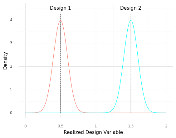
The nominal value for Design 1 is x = 0.5, while the nominal value for Design 2 is x = 1.5. However, parts manufactured according to both designs are subject to manufacturing variability, as depicted by the following densities. Answer the questions under observations below.

mg_1 = gr.marg_mom("norm", mean=+0.5, sd=0.1)
mg_2 = gr.marg_mom("norm", mean=+1.5, sd=0.1)

(
    gr.df_make(x=gr.linspace(0, +2, 100))
    >> gr.tf_mutate(
        y_1=mg_1.d(DF.x),
        y_2=mg_2.d(DF.x),
    )
    
    >> gr.ggplot(gr.aes("x"))
    + gr.annotate("segment", x=+0.5, xend=+0.5, y=0, yend=4.25, linetype="dashed")
    + gr.annotate(
        "text",
        x=+0.5, y=4.5,
        label="Design 1",
    )
    + gr.annotate("segment", x=+1.5, xend=+1.5, y=0, yend=4.25, linetype="dashed")
    + gr.annotate(
        "text",
        x=+1.5, y=4.5,
        label="Design 2",
    )
    + gr.geom_line(gr.aes(y="y_1"), color="salmon")
    + gr.geom_line(gr.aes(y="y_2"), color="cyan")
    
    + gr.theme_minimal()
    + gr.labs(
        x="Realized Design Variable",
        y="Density"
    )
)

<ggplot: (8751230789843)>

Observations

For the following questions, assume that you can measure the Realized Design Variable x with perfect accuracy.

• Suppose you have a part with x == 0.61. Which design specification was this most likely manufactured according to?

  • Design 1

• Suppose you selected a random part of Design 2 off the manufacturing line and found that x == 1.40. Would you be surprised by this?

  • Unsurprising; we can see that x == 1.40 is well-within the distribution around the nominal Design 2 value.

q2 Set up a perturbation model

Implement a model for a perturbed design variable \(x_r\) following

\[x_r = x + \Delta x\]

where \(\Delta x\) is normally distributed with mean \(\mu = 0\) and standard deviation \(\sigma = 0.1\).

Hint 1: To do this, you’ll need to add a function to the model that computes \(x_r\), and a random variable for \(\Delta x\).

Hint 2: The previous exercises e-grama06-fit-univar and e-grama07-fit-multivar cover how to model an uncertain quantity.

## TASK: Implement the model for x_r stated above

md_dx = (
    gr.Model("Perturbation")
    >> gr.cp_vec_function(

        fun=lambda df: gr.df_make(
            x_r=df.x + df.dx,
        ),
        var=["x", "dx"],
        out=["x_r"],
    )
    >> gr.cp_bounds(x=(-1, +1))

    >> gr.cp_marginals(
        dx=gr.marg_mom("norm", mean=0, sd=0.1),
    )
    >> gr.cp_copula_independence()
)

## NOTE: Use this to check your work
gr.eval_sample(md_dx, n=1, df_det="nom")
    
assert \
    'dx' in md_dx.density.marginals.keys(), \
    'No density for dx'
assert \
    md_dx.density.marginals['dx'].d_param['loc'] == 0., \
    "Density for dx has wrong mean"
assert \
    md_dx.density.marginals['dx'].d_param['scale'] == 0.1, \
    "Density for dx has wrong standard deviation"
    

Uncertainty Propagation

Often, we model engineering outcomes deterministically; assuming certain inputs \(x\) are known exactly, we produce a predictable output value \(y\) based on a mathematical model \(y = f(x)\).

For example, we’ve previously looked at a model for the buckling strength of a rectangular plate

\[\sigma_{cr} = k_{cr} \frac{\pi^2 E}{12 (1 - \mu^2)} \left(\frac{t}{b}\right)^2.\]

This is a deterministic model for the buckling strength \(\sigma_{cr}\) that depends on the plate geometry, such as the plate thickness \(t\).

However, if the input values cannot be controlled exactly, it may be more appropriate to think of the model as having perturbed inputs \(x_r = x + \Delta x\). With perturbed inputs, the output is no longer precisely known, but is now subject to uncertainty propagation. We can think of this mathematically as

\[y(x) = f(x_r) = f(x + \Delta x).\]

Where the input that the function “sees” is the perturbed input, rather than the deterministic input. This leads to uncertainty in the output \(y\)—the uncertainty propagates from the input to the output.

Returning to the buckling strength example, if there were manufacturing variability in the plate thickness \(t_r = t + \Delta t\), then there would be uncertainty in the buckling strength

\[\sigma_{cr} = k_{cr} \frac{\pi^2 E}{12 (1 - \mu^2)} \left(\frac{t + \Delta t}{b}\right)^2.\]

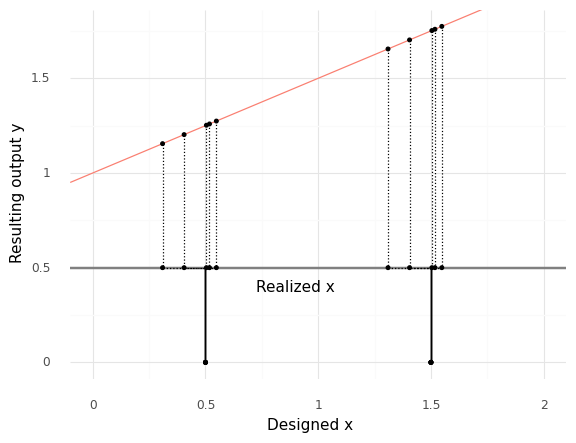
The following images depict uncertainty propagation schematically. First, let’s look at a linear function \(f(x)\).

# NOTE: No need to edit; this illustrates uncertainty propagation
md_line = (
    md_dx
    >> gr.cp_vec_function(
        fun=lambda df: gr.df_make(y=0.5*df.x_r + 1),
        var=["x_r"],
        out=["y"],
    )
)

y_baseboard = 0.5

(
    md_line
    >> gr.ev_sample(
        n=5,
        df_det=gr.df_make(x=(0.5, 1.5)),
        seed=101,
    )
    
    >> gr.ggplot(gr.aes("x_r", "y"))
    + gr.geom_hline(yintercept=y_baseboard, color="grey", size=1)
    + gr.geom_abline(intercept=1, slope=0.5, color="salmon")
    
    + gr.geom_segment(gr.aes(xend="x_r", yend=y_baseboard), linetype="dotted")
    + gr.geom_segment(gr.aes(xend="x", y=y_baseboard, yend=y_baseboard), linetype="dotted")
    + gr.geom_segment(gr.aes(x="x", xend="x", y=0, yend=y_baseboard))
    + gr.geom_point(size=1)
    + gr.geom_point(gr.aes(y=y_baseboard), size=1)
    + gr.geom_point(gr.aes(x="x", y=0), size=1)
    + gr.annotate(
        "text",
        x=0.9,
        y=y_baseboard-0.1,
        label="Realized x",
    )
    
    + gr.scale_x_continuous(limits=(0, 2))
    + gr.theme_minimal()
    + gr.labs(
        x="Designed x",
        y="Resulting output y",
    )
)

<ggplot: (8751231254218)>

Here we have designed values of \(x\) at \(x = 0.5\) and \(x = 1.5\). However, perturbations lead to variability in the realized values \(x_r\), which in turn lead to variability in the output \(y\).

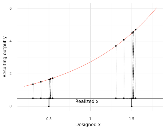
The variability in \(y\) is roughly the same at both designed values \(x\). However, a different function can lead to quite different results.

# NOTE: No need to edit; this illustrates uncertainty propagation
md_exp = (
    md_dx
    >> gr.cp_vec_function(
        fun=lambda df: gr.df_make(y=gr.exp(df.x_r)),
        var=["x_r"],
        out=["y"],
    )
)

y_baseboard = 0.5

(
    md_exp
    >> gr.ev_sample(
        n=5,
        df_det=gr.df_make(x=(0.5, 1.5)),
        seed=101,
    )
    
    >> gr.ggplot(gr.aes("x_r", "y"))
    + gr.geom_hline(yintercept=y_baseboard, color="grey", size=1)
    + gr.geom_line(
        data=md_exp
        >> gr.ev_nominal(df_det=gr.df_make(x=gr.linspace(0.2, 1.8, 100))),
        mapping=gr.aes("x"),
        color="salmon",
    )
    
    + gr.geom_segment(gr.aes(xend="x_r", yend=y_baseboard), linetype="dotted")
    + gr.geom_segment(gr.aes(xend="x", y=y_baseboard, yend=y_baseboard), linetype="dotted")
    + gr.geom_segment(gr.aes(x="x", xend="x", y=0, yend=y_baseboard))
    + gr.geom_point(size=1)
    + gr.geom_point(gr.aes(y=y_baseboard), size=1)
    + gr.geom_point(gr.aes(x="x", y=0), size=1)
    + gr.annotate(
        "text",
        x=0.96,
        y=y_baseboard-0.2,
        label="Realized x",
    )
    
    + gr.theme_minimal()
    + gr.labs(
        x="Designed x",
        y="Resulting output y",
    )
)

<ggplot: (8751230774492)>

Once again we see variability in the realized values. However, note that the variability in the realized output y

q3 Do a sweep with propagated uncertainty

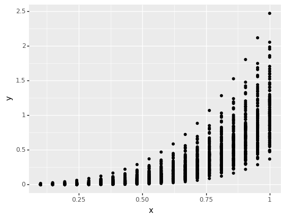
Use your perturbation model md_dx to study how variability propagates through the function

\[y(x) = f(x_r) = x_r^4.\]

Sweep the design variable \(x\) from at least \(0.1\) to \(1.0\), and make sure to use a sufficient number of observations in your random sample. Answer the questions under observations below.

## TASK: Evaluate a sweep with with propagated uncertainty
df_dx = (
    md_dx
    # NOTE: No need to edit; this composes the output function
    # with the perturbation model you implemented above
    >> gr.cp_vec_function(
        fun=lambda df: gr.df_make(y=df.x_r**4),
        var=["x_r"],
        out=["y"],
    )
    

    >> gr.ev_sample(
        n=100,
        df_det=gr.df_make(x=gr.linspace(0.1, 1.0, 20)),
    )
)

## NOTE: Use this to check your work
assert \
    isinstance(df_dx, pd.DataFrame), \
    "df_dx is not a DataFrame; make sure to evaluate md_dx"
assert \
    df_dx.x.min() <= 0.1, \
    "Make sure to sweep to a value as low as x == 0.1"
assert \
    df_dx.x.max() >= 1.0, \
    "Make sure to sweep to a value as high as x == 1.0"
assert \
    len(set(df_dx.x)) >= 10, \
    "Make sure to use a sufficient number of points in your sweep"
assert \
    len(set(df_dx.dx)) >= 100, \
    "Make sure to use a sufficient number of points in your sample"

# Visualize
(
    df_dx
    >> gr.ggplot(gr.aes("x", "y"))
    + gr.geom_point()
)

<ggplot: (8751231026707)>

Observations

• What does the horizontal axis in the plot above represent: The designed value of x or the realized value of x?

  • The horizontal axis in the plot above represents the designed value of x.

• Why is there variability in y?

  • There is variability in y because we are visualizing the designed value of x, while the realized value x_r varies randomly.

• Where (along the horizontal axis) is the variability in y large? Where is it small?

  • The variability is smallest at small values of \(x\), and largest at large values of \(x\).

• What about the underlying function y = f(x) explains the trends in variability you noted above?

  • Since the function is \(y = x_r^4\), variability in \(x_r\) is amplified by the function. A highly quantitative way to think of this is in terms of the derivative \(\frac{dy}{dx_r} = 4 x_r^3 = 4 (x + \Delta x)^3\); note that larger values of the designed value lead to a larger slope in \(y\). (I don’t necessarily expect you to come up with that argument on your own!)

Summarizing variability

Visualizing variability with a scatterplot is a good first-step, but there are more effective ways to summarize variability.

q4 Summarize variability across a sweep

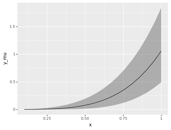
Summarize the variability in \(y\) at each value of \(x\) by computing the mean y_mu, the 5% quantile y_lo, and the 95% quantile y_up. Answer the questions under observations below.

df_dx_summary = (
    df_dx

    >> gr.tf_group_by(DF.x)
    >> gr.tf_summarize(
        y_lo=gr.quant(DF.y, p=0.05),
        y_mu=gr.mean(DF.y),
        y_up=gr.quant(DF.y, p=0.95),
    )
    ## NOTE: Clean up the grouping
    >> gr.tf_ungroup()
)

## NOTE: No need to edit; use this to check your work
assert \
    set(df_dx.x) == set(df_dx_summary.x), \
    "Incorrect grouping for df_dx_summary"
assert \
    "y_lo" in df_dx_summary.columns, \
    "Make sure to compute a lower quantile y_lo"
assert \
    "y_up" in df_dx_summary.columns, \
    "Make sure to compute an upper quantile y_up"
# Check the quantiles
df_dx_check = (
    df_dx
    >> gr.tf_left_join(df_dx_summary, by="x")
    >> gr.tf_filter(DF.x == gr.min(DF.x))
    >> gr.tf_summarize(
        p_lo=gr.pr(DF.y <= DF.y_lo),
        p_up=gr.pr(DF.y <= DF.y_up),
    )
)
assert \
    abs(df_dx_check.p_lo[0] - 0.05) < 1e-3, \
    "Lower quantile value is incorrect"
assert \
    abs(df_dx_check.p_up[0] - 0.95) < 1e-3, \
    "Upper quantile value is incorrect"

(
    df_dx_summary
    >> gr.ggplot(gr.aes("x"))
    + gr.geom_ribbon(
        mapping=gr.aes(ymin="y_lo", ymax="y_up"),
        alpha=1/3,
    )
    + gr.geom_line(gr.aes(y="y_mu"))
)

<ggplot: (8751230919190)>

Observations

Note: This plot uses geom_ribbon(), which takes the aesthetics ymin and ymax. A ribbon is a useful way to visualize a region bounded by lower and upper values, such as quantiles!

• Contrast this plot with the scatterplot from q3: What can you see in this ribbon plot that is harder to see in the scatterplot?

  • Some examples: We can see the mean trend quite clearly, while the mean trend is harder to judge by eye in the scatterplot. We can also see particular quantiles; if we wanted to make decisions based on the middle 90% of the data, these would be ideal bounds to use. If we wanted to use a different fraction of the data (say, 99%) we could adjust the quantiles (say, 0.005 and 0.995).

Designing for uncertainty

We’ve seen that uncertainty can propagate through systems—what can we do about that? There are various ways we can design systems to mitigate the effects of uncertainty: We can seek robust designs, we can explicitly design for reliability, and we can set tolerances to achieve design targets.

Robustness

Sometimes, the best nominal performance does not result in the overall “best” design. Since uncertainty can propagate, a design that is highly sensitive to input variability can fail to live up to the promise of its best nominal performance. The following example will guide you through thinking about designs that are robust, in the sense that they are resistant to uncertainty.

## NOTE: No need to edit; this sets up a model with
## a perturbed input and a complex output function
md_poly = (
    gr.Model("Polynomial")
    >> gr.cp_vec_function(
        fun=lambda df: gr.df_make(
            x_r=df.x + df.dx
        ),
        var=["x", "dx"],
        out=["x_r"],
        name="Realized design"
    )
    >> gr.cp_vec_function(
        fun=lambda df: gr.df_make(
            y=(df.x_r + 0.6) 
             *(df.x_r + 0.4) 
             *(df.x_r - 0.65)
             *(df.x_r - 0.55)
             *13.5 * (1 + gr.exp(8.0 * df.x_r))
        ),
        var=["x_r"],
        out=["y"],
        name="Realized output"
    )
    >> gr.cp_bounds(x=(-1, +1))
    >> gr.cp_marginals(dx=gr.marg_mom("norm", mean=0, sd=0.03))
    >> gr.cp_copula_independence()
)

q5 Interpret this plot

Run the following code and inspect the plot. Answer the questions under observations below.

## NOTE: No need to edit; run and inspect
# Evaluate model without uncertainty
df_poly_nom = (
    md_poly
    >> gr.ev_nominal(
        df_det=gr.df_make(x=gr.linspace(-1, +1, 100)),
    )
)

# Evaluate with uncertainty, take quantiles
df_poly_mc = (
    md_poly
    >> gr.ev_sample(
        df_det=gr.df_make(x=gr.linspace(-1, +1, 100)),
        n=40,
        seed=101,
    )
    >> gr.tf_group_by("x")
    >> gr.tf_summarize(
        y_lo=gr.quant(DF.y, p=0.05),
        y_mu=gr.median(DF.y),
        y_up=gr.quant(DF.y, p=0.95),
    )
    >> gr.tf_ungroup()
)

# Visualize
(
    df_poly_mc
    >> gr.tf_mutate(source="Quantiles")
    >> gr.ggplot(gr.aes("x"))
    + gr.geom_line(
        data=df_poly_nom
        >> gr.tf_mutate(source="Nominal"),
        mapping=gr.aes(y="y"),
    )
    + gr.geom_ribbon(
        mapping=gr.aes(ymin="y_lo", ymax="y_up"),
        alpha=1/3,
    )
    
    + gr.scale_y_continuous(breaks=(-10, -5, 0, +5, +10, +15, +20))
    + gr.coord_cartesian(ylim=(-10, 20))
    + gr.theme_minimal()
    + gr.guides(color=None)
    + gr.labs(
        x="Designed input value x",
        y="Realized output value y",
    )
)

<ggplot: (8751230981578)>

Observations

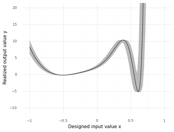
For this example, lower values of y are better. The solid curve depicts the Nominal output value, while the shaded region visualizes the 5% to 95% quantiles.

• Approximately, what is the lowest value y value the Nominal curve (solid curve) achieves across the values of x depicted above?

  • \(y_{\min} \approx -5\)

• Approimately, what is the value of y for the Nominal curve at x = -0.5?

  • \(y(x = -0.5) \approx 0\)

• Note the spread between the Quantiles at \(x \approx 0.6\). Approximately what range of y values would you expect to result from releated manufacturing at \(x \approx 0.6\)?

  • \(y \in [-5, 1]\)

• Note the spread between the Quantiles at \(x \approx -0.5\). Approximately what range of y values would you expect to result from releated manufacturing at \(x \approx -0.5\)?

  • \(y \in [0, 0]\)

• Suppose you plan to manufacture many parts according to this process, test all specimens, and choose the best 5%. Which design (value of x) would you pick, and why?

  • I would choose \(x = 0.6\) for the design, as we would likely see a large number of highly negative (desirable) values. Post-manufacturing selection would allow us to collect a subset of highly-performing specimens.

• Suppose you plan to manufacture many parts according to this process, all of which must work at an acceptable level. Which design (value of x) would you pick, and why?

  • I would choose \(x = -0.5\) for the design, as we need the performance of the parts to be consistent.

Reliability

While robustness is about reducing variability, reliability is about avoiding unwanted failures. A reliable design is a design that has a low probability of failure. With a model for a system and its uncertainties, we can use uncertainty propagation to quantify the probability of failure, and use the model to test the reliability of different designs.

For the remainder of this exercise, let’s use the cantilever beam model as an example.

from grama.models import make_cantilever_beam
md_beam = make_cantilever_beam()
md_beam

model: Cantilever Beam

  inputs:
    var_det:
      w: [2, 4]
      t: [2, 4]

    var_rand:
      H: (+1) norm, {'mean': '5.000e+02', 's.d.': '1.000e+02', 'COV': 0.2, 'skew.': 0.0, 'kurt.': 3.0}
      V: (+1) norm, {'mean': '1.000e+03', 's.d.': '1.000e+02', 'COV': 0.1, 'skew.': 0.0, 'kurt.': 3.0}
      E: (+0) norm, {'mean': '2.900e+07', 's.d.': '1.450e+06', 'COV': 0.05, 'skew.': 0.0, 'kurt.': 3.0}
      Y: (-1) norm, {'mean': '4.000e+04', 's.d.': '2.000e+03', 'COV': 0.05, 'skew.': 0.0, 'kurt.': 3.0}

    copula:
      Independence copula

  functions:
      cross-sectional area: ['w', 't'] -> ['c_area']
      limit state: stress: ['w', 't', 'H', 'V', 'E', 'Y'] -> ['g_stress']
      limit state: displacement: ['w', 't', 'H', 'V', 'E', 'Y'] -> ['g_disp']

q6 Compare the reliability of designs

Estimate the probability of failure due to stress for the following cantilever beam designs. Make sure to compute lower and upper confidence interval bounds for your estimate, and choose a large enough sample size so that the CI for the designs do not overlap. Answer the questions under observations below.

Hint: Remember that we learned about estimating probabilities of failure (and related confidence intervals) in e-stat05-CI.

## TASK: Estimate the reliability for the following beam designs

# NOTE: No need to edit; evaluate these designs
df_beam_designs = gr.df_make(
    design=["Wide", "Tall", "Square"],
    w=[4, 2, gr.sqrt(8)],
    t=[2, 4, gr.sqrt(8)],
)

## TASK: Complete the following code
df_beam_results = (
    md_beam

    >> gr.ev_sample(
        n=1e4, 
        df_det=df_beam_designs, 
        seed=101,
    )
    >> gr.tf_group_by(DF.design)
    >> gr.tf_summarize(
        pof_lo=gr.pr_lo(DF.g_stress <= 0),
        pof_mu=gr.pr(DF.g_stress <= 0),
        pof_up=gr.pr_up(DF.g_stress <= 0),
    )
    >> gr.tf_ungroup()
)

print(df_beam_results)

## NOTE: No need to edit below; use this to check your work
assert \
    isinstance(df_beam_results, pd.DataFrame), \
    "df_beam_results is not a DataFrame; make sure to evaluate and summarize"
assert \
    {"Square", "Tall", "Wide"} == set(df_beam_results.design), \
    "df_beam_results does not contain rows for each design; make sure to group appropriately"
assert \
    "pof_lo" in df_beam_results.columns, \
    "CI lower bound pof_lo not found in df_beam_results; make sure to compute a lower CI bound"
assert \
    "pof_up" in df_beam_results.columns, \
    "CI upper bound pof_up not found in df_beam_results; make sure to compute an upper CI bound"
assert \
    df_beam_results[df_beam_results.design=="Tall"].pof_up.values[0] < \
    df_beam_results[df_beam_results.design=="Square"].pof_lo.values[0], \
    "CI overlap; make sure to use a sufficiently large sample size"
assert \
    df_beam_results[df_beam_results.design=="Square"].pof_up.values[0] < \
    df_beam_results[df_beam_results.design=="Wide"].pof_lo.values[0], \
    "CI overlap; make sure to use a sufficiently large sample size"

eval_sample() is rounding n...
   design    pof_lo  pof_mu    pof_up
0  Square  0.473439  0.4863  0.499179
1    Tall  0.282503  0.2941  0.305970
2    Wide  0.928253  0.9349  0.940971

Observations

• Which design has the lowest probability of failure?

  • The Tall design has the lowest probability of failure.

• All of these designs have the same cross-sectional area; they vary from wide to square to tall in their rectangular cross-section shape. Based on the result above, does the nominal width or tallness of the cross-section seem to be more important for safe operation?

  • Tallness seems to be most important, based on these results.

Setting Tolerances

Once we represent uncertainty in a model, we can make modifications to that model to make quantitative statements about system performance. For instance, modeling the tolerances for a manufactured component will allow us to test different tolerance scenarios. This can help us decide whether to ask manufacturing to tighten specific tolerances.

The following code adds a perturbation model for tolerances on the width and tallness of the cantilever beam. You’ll use this model below to test different tolerance scenarios.

## NOTE: NO need to edit; this adds tolerances to the cantilever beam model
md_beam_tolerances = (
    gr.Model()
    >> gr.cp_vec_function(
        fun=lambda df: gr.df_make(
            w=df.w0 + df.dw,
            t=df.t0 + df.dt,
        ),
        var=["w0", "t0", "dw", "dt"],
        out=["w", "t"],
        name="Design perturbations",
    )
    ## NOTE: gr.cp_md_det() is an advanced tool I'm using to
    ## avoid re-defining the entire beam model. You could
    ## accomplish the same thing with gr.cp_vec_function()
    ## and the beam equations
    >> gr.cp_md_det(md_beam)
    ## Define the input space
    >> gr.cp_bounds(
        w0=(2, 4),
        t0=(2, 4),
    )
    >> gr.cp_marginals(
        # Uncertainties from the original model
        H=gr.marg_mom("norm", mean=500, sd=100),
        V=gr.marg_mom("norm", mean=1000, sd=100),
        E=gr.marg_mom("norm", mean=2.9e7, sd=1.45e6),
        Y=gr.marg_mom("norm", mean=40000, sd=2000),
        # Variability in width and tallness
        dw=gr.marg_mom("uniform", mean=0, sd=1e-1),
        dt=gr.marg_mom("uniform", mean=0, sd=1e-1),
    )
    >> gr.cp_copula_independence()
)
md_beam_tolerances 

/home/zach/Git/py_grama/grama/marginals.py:336: RuntimeWarning: divide by zero encountered in double_scalars

model: None

  inputs:
    var_det:
      t0: [2, 4]
      w0: [2, 4]

    var_rand:
      H: (+0) norm, {'mean': '5.000e+02', 's.d.': '1.000e+02', 'COV': 0.2, 'skew.': 0.0, 'kurt.': 3.0}
      V: (+0) norm, {'mean': '1.000e+03', 's.d.': '1.000e+02', 'COV': 0.1, 'skew.': 0.0, 'kurt.': 3.0}
      E: (+0) norm, {'mean': '2.900e+07', 's.d.': '1.450e+06', 'COV': 0.05, 'skew.': 0.0, 'kurt.': 3.0}
      Y: (+0) norm, {'mean': '4.000e+04', 's.d.': '2.000e+03', 'COV': 0.05, 'skew.': 0.0, 'kurt.': 3.0}
      dw: (+0) uniform, {'mean': '0.000e+00', 's.d.': '1.000e-01', 'COV': inf, 'skew.': 0.0, 'kurt.': 1.8}
      dt: (+0) uniform, {'mean': '0.000e+00', 's.d.': '1.000e-01', 'COV': inf, 'skew.': 0.0, 'kurt.': 1.8}

    copula:
      Independence copula

  functions:
      Design perturbations: ['w0', 't0', 'dw', 'dt'] -> ['w', 't']
      Cantilever Beam: ['w', 'Y', 't', 'V', 'E', 'H'] -> ['c_area', 'g_stress', 'g_disp']

First, let’s evaluate the baseline tolerance model to assess the probability of failure for a few designs.

## NOTE: No need to edit; this estimates probabilities of failure
## for the three designs
df_beam_baseline = (
    md_beam_tolerances
    >> gr.ev_sample(
        n=1e4, 
        df_det=gr.df_make(
            design=["Wide", "Tall", "Square"],
            w0=[4, 2, gr.sqrt(8)],
            t0=[2, 4, gr.sqrt(8)],
        ), 
        seed=101,
    )
    >> gr.tf_group_by(DF.design)
    >> gr.tf_summarize(
        pof_lo=gr.pr_lo(DF.g_stress <= 0),
        pof_mu=gr.pr(DF.g_stress <= 0),
        pof_up=gr.pr_up(DF.g_stress <= 0),
    )
    >> gr.tf_ungroup()
    >> gr.tf_mutate(model="Baseline")
)
df_beam_baseline

eval_sample() is rounding n...

	design	pof_lo	pof_mu	pof_up	model
0	Square	0.479931	0.4928	0.505678	Baseline
1	Tall	0.325530	0.3376	0.349885	Baseline
2	Wide	0.868392	0.8771	0.885308	Baseline

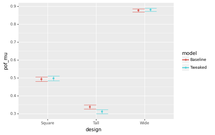
q7 Recommend reasonable tolerances

Adjust the manufacturing tolerances to find desirable manufacturing targets. Answer the questions under observations below.

## TASK: Tweak the tolerances

df_beam_tweaked = (
    md_beam_tolerances
    >> gr.cp_marginals(

        dw=gr.marg_mom("uniform", mean=0, sd=1e-3), # Reduce width tolerance
#         dt=gr.marg_mom("uniform", mean=0, sd=1e-3), # Reduce tallness tolerance
    )
    ## NOTE: No need to edit below; this analyzes your model
    >> gr.ev_sample(
        n=1e4, 
        df_det=gr.df_make(
            design=["Wide", "Tall", "Square"],
            w0=[4, 2, gr.sqrt(8)],
            t0=[2, 4, gr.sqrt(8)],
        ), 
        seed=101,
    )
    >> gr.tf_group_by(DF.design)
    >> gr.tf_summarize(
        pof_lo=gr.pr_lo(DF.g_stress <= 0),
        pof_mu=gr.pr(DF.g_stress <= 0),
        pof_up=gr.pr_up(DF.g_stress <= 0),
    )
    >> gr.tf_ungroup()
    >> gr.tf_mutate(model="Tweaked")
)

## NOTE: This will visualize your results with
## a comparison against the baseline model
(
    df_beam_baseline
    >> gr.tf_bind_rows(df_beam_tweaked)
    >> gr.ggplot(gr.aes("design", color="model"))
    + gr.geom_errorbar(
        gr.aes(ymin="pof_lo", ymax="pof_up"),
        position=gr.position_dodge(width=0.5),
    )
    + gr.geom_point(
        gr.aes(y="pof_mu"), 
        position=gr.position_dodge(width=0.5),
    )
)

eval_sample() is rounding n...

<ggplot: (8751231278427)>

Observations

Note: It’s likely you’ll need to tweak and re-run the analysis above to answer these questions:

• Suppose you could reduce the standard deviation sd to 1e-3 for both the width dw and tallness dt tolerances. Which designs would this benefit?

  • Reducing the tolerances for both dw and dt would benefit the Tall design; it would significantly reduce the probability of failure. The same move would not benefit the Square design at all (the CI’s overlap; no difference in their performance). Surprisingly, making the tolerances narrower would actually make the unsafe Wide design even more likely to fail.

• Consider the Tall design. Suppose it were only economical to reduce one of the tolerances: either for dw or dt. Which would be the more valuable tolerance to reduce?

  • Reducing the tolerance for dw is more valuable; in fact reducing the tolerance for dt does not result in a significant change for pof_mu.

• In q6 Compare the reliability of designs, you answered the question “does the nominal width or tallness of the cross-section seem to be more important for safe operation?” How does your answer immediately above compare with your past answer?

  • Surprisingly, the nominal thickness t0 matters most for safe operation, but reducing the tolerance for dw most reduces the failure rate for the Thick design.