Grama: Exploratory Model Analysis

Purpose: Once we’ve built a grama model, we can use a variety of tools to make sense of the model. However, as we saw with exploratory data analysis (EDA), we need both tools and a mindset to make sense of data. This exercise is about an analogous approach to sense-making with models: exploratory model analysis (EMA).

Core Idea: Curiosity and Skepticism

Remember the core principles of EDA:

1. Curiosity: Generate lots of ideas and hypotheses about your data.

2. Skepticism: Remain unconvinced of those ideas, unless you can find credible patterns to support them.

We can apply these same principles when studying a model; a process called exploratory model analysis. However, when studying a model, we have the means to more immediately test our hypotheses: We can evaluate the model to generate new data as we’re carrying out our exploration!

These ideas can be a little abstract, so let’s illustrate them with a concrete example.

Setup

import grama as gr
import pandas as pd
DF = gr.Intention()
%matplotlib inline

Running Example: Circuit model

The following code initializes a model for a parallel RLC circuit. I’m not expecting you to know any circuit theory; in fact, I chose this model because you’re unlikely to know much about this system. We will use exploratory model analysis techniques to learn something about this model.

from grama.models import make_prlc_rand
md_circuit = make_prlc_rand()

Basic Facts

Before we start exploring a model, we should first understand the basic facts about that model. This is most easily done in grama by printing the model’s summary:

q1 Model summary

Print the model summary for md_circuit. Answer the questions under observations below.

md_circuit 
# solution-end

/Users/zach/Git/py_grama/grama/marginals.py:336: RuntimeWarning: divide by zero encountered in double_scalars

model: RLC with component tolerances

  inputs:
    var_det:
      L: [1e-09, 0.001]
      R: [0.001, 1.0]
      C: [0.001, 100]

    var_rand:
      dR: (+0) uniform, {'mean': '0.000e+00', 's.d.': '3.000e-02', 'COV': inf, 'skew.': 0.0, 'kurt.': 1.8}
      dL: (+0) uniform, {'mean': '0.000e+00', 's.d.': '6.000e-02', 'COV': inf, 'skew.': 0.0, 'kurt.': 1.8}
      dC: (+0) uniform, {'mean': '3.000e-01', 's.d.': '2.900e-01', 'COV': 0.96, 'skew.': 0.0, 'kurt.': 1.8}

    copula:
      Independence copula

  functions:
      f0: ['R', 'dR', 'L', 'dL', 'C', 'dC'] -> ['Rr', 'Lr', 'Cr']
      f1: ['Lr', 'Cr'] -> ['omega0']
      parallel RLC: ['omega0', 'Rr', 'Cr'] -> ['Q']

Observations

• Compare the variability (measured by standard deviation) of the three random variables. Which is most variable?

  • dC has the largest variability, with sd = 0.29, as compared with dR (sd = 0.03) and dL (sd = 0.06).

Model context

The symbols above don’t tell us anything about what the model quantities mean. Here are some basic facts on the quantities in the model

Variable	I/O	Description
L	Input	Nominal inductance
R	Input	Nominal resistance
C	Input	Nominal capacitance
dL	Input	Percent error on inductance
dR	Input	Percent error on resistance
dC	Input	Percent error on capacitance
omega0	Output	Natural frequency
Q	Output	Quality factor

The deterministic variables L, R, C are the designed component values; these are selected by a circuit designer to achieve a desired performance.

The random variables dL, dR, dC are perturbations to the designed component values. These random perturbations model the variability we would see in production, as manufactured components exhibit real variability.

The output omega0 is the natural frequency; depending on the use-case, a designer would want to achieve a particular omega0. Thus having omega0 lie close to some target value is desirable.

The output Q is the quality factor; a larger Q corresponds to a more “selective” circuit. Put differently, a higher Q helps the circuit reject unwanted signals.

Inputs

First, let’s get a sense for how the inputs of the model vary.

q2 Overview of inputs

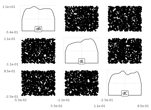
Generate a random sample from the model at its nominal deterministic values, and visualize all of the random inputs. Answer the questions under observations below.

Hint: You should be using gr.ev_sample() for this task. A particular keyword argument with gr.ev_sample() will allow you to generate the appropriate plot using gr.pt_auto().

(
    md_circuit
    >> gr.ev_sample(n=1e3, df_det="nom", skip=True)
    >> gr.pt_auto()
)

eval_sample() is rounding n...
Design runtime estimates unavailable; model has no timing data.
Calling plot_scattermat....

/Users/zach/Git/py_grama/grama/plot_auto.py:234: UserWarning: Matplotlib is currently using module://matplotlib_inline.backend_inline, which is a non-GUI backend, so cannot show the figure.

Observations

Note: If you can’t reliably make out the shapes of the distributions, try increasing n.

• What shape of distribution does each random input have?

  • All three distributions are uniform; we can see that from the marginals (along the diagonal), and from the model summary information above.

• What kind of dependency do the random inputs exhibit?

  • All three inputs are mutually independent; we can see that from the scatterplots (off-diagonal panels), and from the model summary information above (independence copula).

Hypothesis: Same Variability

Since the random perturbations dL, dR, dC are mutually independent, we should see the same variability regardless of the circuit component values.

You’ll assess this hypothesis in the next task.

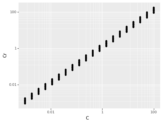
q3 Compare designed and realized values

The following plot shows the designed and realized capacitance values. Answer the questions under observations below.

Hint: Remember that you can add gr.scale_x_log10() and gr.scale_y_log10() to a ggplot to change to a log-log scale.

# TASK: Inspect the following plot
(
    # NOTE: No need to edit this part of the code
    md_circuit
    >> gr.ev_sample(
        n=20,
        df_det=gr.df_make(
            R=1e-1,
            L=1e-5,
            C=gr.logspace(-3, 2, 20)
        )
    )
    # Visualize
    >> gr.ggplot(gr.aes("C", "Cr"))
    + gr.geom_point()
    + gr.scale_x_log10()
    + gr.scale_y_log10()
)

<ggplot: (8763311150466)>

Observations

• Consider the hypothesis we should see the same variability regardless of the circuit component values. Is this hypothesis true?

  • This really depends on how we define “same variability”; since the variability is proportional to the component values (defined in terms of \(\pm\) a fixed percentage), the variability is greater for larger component values. However, the percentage variability is consistent regardless of the component value; this is easiest to see on a log-log scale.

Outputs

Next, we’ll study the outputs of the model “on their own”; that is, we’re not yet going to look at the input-to-output relationships.

q4 Nominal outputs

Evaluate the model at its nominal input values.

## TODO: Evaluate the model at its nominal input values
df_nominal = (
    md_circuit
    >> gr.ev_nominal(df_det="nom")
)

# NOTE: Use this to check your work
assert \
    isinstance(df_nominal, pd.DataFrame), \
    "df_nominal is not a DataFrame; did you evaluate the model?"

df_nominal

	dR	dL	dC	L	R	C	Q	Rr	omega0	Lr	Cr
0	0.0	0.0	0.3	0.0005	0.5005	50.0005	180.458653	0.5005	5.546971	0.0005	65.00065

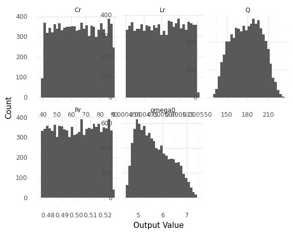
q5 Overview of outputs

Generate a random sample from the model at its nominal deterministic values, and visualize the distribution of outputs. Answer the questions under observations below.

Hint: This is a lot like qX Overview of inputs. You should only need to use gr.ev_sample() and gr.pt_auto().

(
    md_circuit

    >> gr.ev_sample(n=1e4, df_det="nom")
    >> gr.pt_auto()
)

eval_sample() is rounding n...
Calling plot_hists....

/Users/zach/opt/anaconda3/envs/evc/lib/python3.9/site-packages/plotnine/utils.py:371: FutureWarning: The frame.append method is deprecated and will be removed from pandas in a future version. Use pandas.concat instead.
/Users/zach/opt/anaconda3/envs/evc/lib/python3.9/site-packages/plotnine/facets/facet.py:390: PlotnineWarning: If you need more space for the x-axis tick text use ... + theme(subplots_adjust={'wspace': 0.25}). Choose an appropriate value for 'wspace'.
/Users/zach/opt/anaconda3/envs/evc/lib/python3.9/site-packages/plotnine/facets/facet.py:396: PlotnineWarning: If you need more space for the y-axis tick text use ... + theme(subplots_adjust={'hspace': 0.25}). Choose an appropriate value for 'hspace'

<ggplot: (8763303613248)>

Observations

Note: If you can’t reliably make out the shapes of the distributions, try increasing n.

• What distribution shapes do the realized component values Lr, Rr, Cr have?

  • These are all uniform distributions

• What distribution shape does the output Q have?

  • This distribution is a bit bell-shaped, but it has a much flatter top and narrower tails than a gaussian.

• What distribution shape does the output omega0 have?

  • This distribution is strongly asymmetric, with a longer right tail (right skew).

Hypothesis: Nominal Outputs are Likely Outputs

Here’s something we might intuitively expect:

The nominal model outputs should be more likely output values.

You’ll assess this hypothesis multiple different ways in the following tasks.

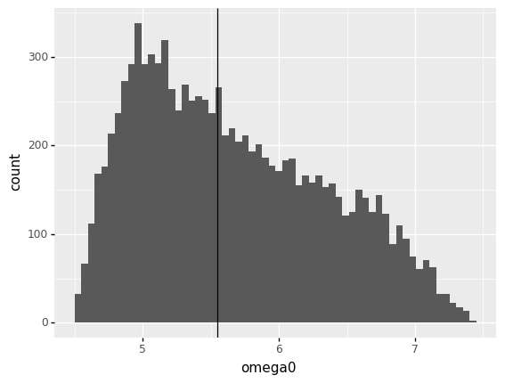
q6 Compare distribution and nominal values for omega0

Create a plot that visualizes both a distribution of omega0 and the nominal output value of omega0. Answer the questions under observations below.

Hint: One good way to do this is with a histogram and a vertical line.

(
    md_circuit
    >> gr.ev_sample(n=1e4, df_det="nom")
    >> gr.ggplot(gr.aes("omega0"))
    + gr.geom_histogram(bins=60)
    + gr.geom_vline(
        data=df_nominal,
        mapping=gr.aes(xintercept="omega0")
    )
)

eval_sample() is rounding n...

<ggplot: (8763311154990)>

Observations

• How does the hypothesis The nominal model outputs should be more likely output values hold up for omega0?

  • For omega0 this hypothesis is somewhat false; the most likely value for omega0 is around 5.0, but the nominal value is closer to 5.5. The nominal output value is certainly not the most unlikely value, though.

q7 Density of outputs

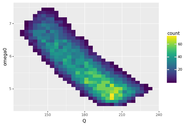
Visualize a random sample of Q and omega0 with a 2d bin plot. Increase the sample size n to get a “full” plot. Answer the questions under observations below.

(
    md_circuit

    >> gr.ev_sample(n=1e4, df_det="nom")
    >> gr.ggplot(gr.aes("Q", "omega0"))
    + gr.geom_bin2d()
)

eval_sample() is rounding n...

<ggplot: (8763303531936)>

Observations

• Briefly describe the distribution of realized performance (values of Q and omega0).

  • The distribution is oddly rectangular, with fairly “sharp” square sides. The distribution seems to end abruptly; there are exactly zero counts outside the “curved rectangle”. The values of Q and omega0 are negatively correlated; when Q is larger omega0 tends to be smaller. The distribution is also asymmetric; note that highest count (brightest fill color) is not in the center, but rather towards the bottom-right.

q8 Compare nominal with distribution

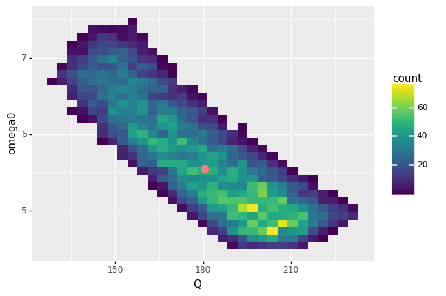
Add a point for the nominal output values to the following plot. Answer the questions under observations below.

## NOTE: You don't need to touch most of this code; 
## just the line indicated below
(
    md_circuit
    >> gr.ev_sample(n=1e4, df_det="nom")
    
    >> gr.ggplot(gr.aes("Q", "omega0"))
    + gr.geom_bin2d()
    + gr.geom_point(

        data=df_nominal,
        color="salmon",
        size=4,
    )
)

eval_sample() is rounding n...

<ggplot: (8763311157447)>

Observations

The nominal design (red point) represents the predicted performance if we assume the nominal circuit component values.

• How does the distribution of real circuit performance (values of Q, omega0) compare with the nominal performance?

  • The distribution of real performance is quite large, and not at all symmetric about the nominal performance. The values Q and omega0 exhibit negative correlation: when Q is larger omega0 tends to be smaller.

• Is the most likely performance (values of Q, omega0) the same as the nominal performance? (“Most likely” is where count is the largest.)

  • No; the most likely performance is at a larger value of Q and smaller value of omega0.

• Assume that another system depends on the particular values of Q and omega0 provided by this system. Would it be safe to assume the performance is within 1% of the nominal performance?

  • No; we see variability in Q and omega0 far greater than 1%!

Input-to-output Relationships

Now that we have a sense of both the inputs and outputs of the model, let’s do some exploration to see how the two are related.

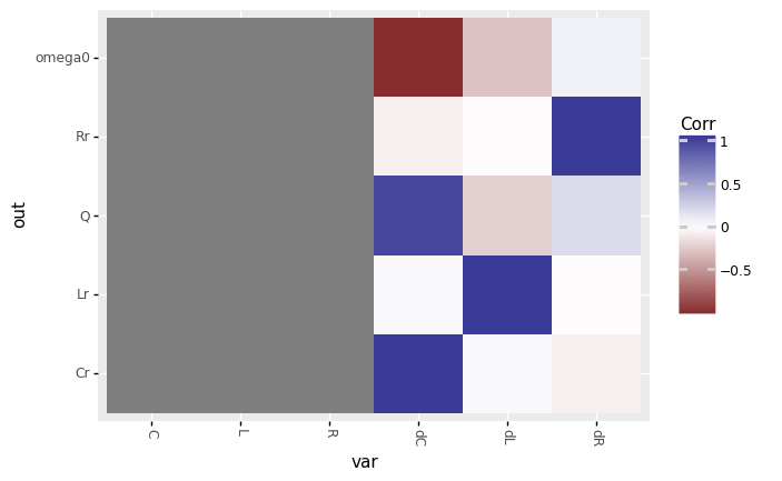
q9 Correlation tile plot

Use the routine tf_iocorr() to transform the data from ev_sample() into input-to-output correlations. The pt_auto() routine will automatically plot those correlations as colors on a tile plot. Study the correlation tile plot, and answer the questions under observations below.

Note: You’re going to see a ton of warnings when you run tf_iocorr() on the data; you’ll think about what those mean in the questions below.

(
    ## NOTE: No need to edit the call to ev_sample()
    md_circuit
    >> gr.ev_sample(
        n=1e3, 
        df_det="nom",
    )

    >> gr.tf_iocorr()
    ## NOTE: No need to edit; pt_auto will automatically
    ## adjust the plot to use the correlation data
    >> gr.pt_auto()
)

eval_sample() is rounding n...
Calling plot_corrtile....

/Users/zach/opt/anaconda3/envs/evc/lib/python3.9/site-packages/scipy/stats/_stats_py.py:4068: PearsonRConstantInputWarning: An input array is constant; the correlation coefficient is not defined.
/Users/zach/opt/anaconda3/envs/evc/lib/python3.9/site-packages/scipy/stats/_stats_py.py:4068: PearsonRConstantInputWarning: An input array is constant; the correlation coefficient is not defined.
/Users/zach/opt/anaconda3/envs/evc/lib/python3.9/site-packages/scipy/stats/_stats_py.py:4068: PearsonRConstantInputWarning: An input array is constant; the correlation coefficient is not defined.
/Users/zach/opt/anaconda3/envs/evc/lib/python3.9/site-packages/scipy/stats/_stats_py.py:4068: PearsonRConstantInputWarning: An input array is constant; the correlation coefficient is not defined.
/Users/zach/opt/anaconda3/envs/evc/lib/python3.9/site-packages/scipy/stats/_stats_py.py:4068: PearsonRConstantInputWarning: An input array is constant; the correlation coefficient is not defined.
/Users/zach/opt/anaconda3/envs/evc/lib/python3.9/site-packages/scipy/stats/_stats_py.py:4068: PearsonRConstantInputWarning: An input array is constant; the correlation coefficient is not defined.
/Users/zach/opt/anaconda3/envs/evc/lib/python3.9/site-packages/scipy/stats/_stats_py.py:4068: PearsonRConstantInputWarning: An input array is constant; the correlation coefficient is not defined.
/Users/zach/opt/anaconda3/envs/evc/lib/python3.9/site-packages/scipy/stats/_stats_py.py:4068: PearsonRConstantInputWarning: An input array is constant; the correlation coefficient is not defined.
/Users/zach/opt/anaconda3/envs/evc/lib/python3.9/site-packages/scipy/stats/_stats_py.py:4068: PearsonRConstantInputWarning: An input array is constant; the correlation coefficient is not defined.
/Users/zach/opt/anaconda3/envs/evc/lib/python3.9/site-packages/scipy/stats/_stats_py.py:4068: PearsonRConstantInputWarning: An input array is constant; the correlation coefficient is not defined.
/Users/zach/opt/anaconda3/envs/evc/lib/python3.9/site-packages/scipy/stats/_stats_py.py:4068: PearsonRConstantInputWarning: An input array is constant; the correlation coefficient is not defined.
/Users/zach/opt/anaconda3/envs/evc/lib/python3.9/site-packages/scipy/stats/_stats_py.py:4068: PearsonRConstantInputWarning: An input array is constant; the correlation coefficient is not defined.
/Users/zach/opt/anaconda3/envs/evc/lib/python3.9/site-packages/scipy/stats/_stats_py.py:4068: PearsonRConstantInputWarning: An input array is constant; the correlation coefficient is not defined.

<ggplot: (8763303642555)>

Observations

• The verb tf_iocorr() should throw a ton of warnings. What are these messages warning you about? Based on the colors in the plot, which correlations are not defined?

  • The warnings are for input array is constant; some of the values do not vary. Based on the plot, we can see that all correlations involving L, R, C are not defined.

• Do we have any information on how the outputs omega0 and Q depend on the deterministic inputs L, R, C? How does this relate to the warnings we saw above?

  • No; the correlations between the outputs omega0 and Q and inputs L, R, C are invalid. This is related to the warnings because L, R, C are each held at constant values. This is because we set df_det="nom" in the sample above; there is no variability in the inputs L, R, C by which to judge correlation with the outputs.

• Based on the available information: Which inputs does omega0 depend on? How do those inputs affect omega0?

  • omega0 depends on dC and dL; from this we can guess that is also depends on C and L. omega0 is strongly negatively correlated with dC, and weakly negatively correlated with dL.

• Based on the available information: Which inputs does Q depend on? How do those inputs affect Q?

  • Q depends on all of dC, dL, and dR; from this we can guess that it also depends on C, L, R. Q is strongly positively correlated with dC, weakly positively correlated with dR, and weakly negatively correlated with dL.

Hypothesis: dR has no effect on omega0

Based on the correlation tile plot above, we can formulate the following hypothesis:

The variability in the resistance dR has no effect on the natural frequency omega0.

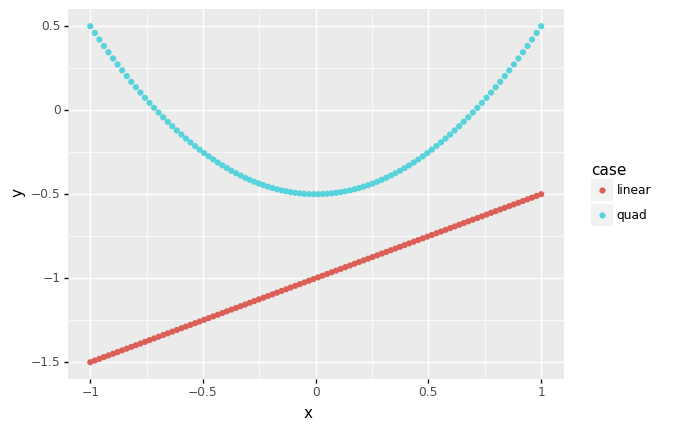
While this may seem obvious, it’s important to keep in mind that correlation is a crude measure of dependency. For instance, the following code generates X, Y pairs that have a deterministic dependency, but very different correlation values:

## NOTE: No need to edit; run and inspect
# Generate data
df_example = (
    gr.df_make(x=gr.linspace(-1, +1, 100))
    >> gr.tf_mutate(
        y_linear=0.5 * DF.x - 1,
        y_quad=1.0 * DF.x**2 - 0.5,
    )
)

# Compute correlation coefficients
print(
    df_example
    >> gr.tf_summarize(
        corr_linear=gr.corr(DF.x, DF.y_linear),
        corr_quad=gr.corr(DF.x, DF.y_quad),
    )
)

# Visualize
(
    df_example
    >> gr.tf_pivot_longer(
        columns=["y_linear", "y_quad"],
        names_to=[".value", "case"],
        names_sep="_",
    )
    >> gr.ggplot(gr.aes("x", "y", color="case"))
    + gr.geom_point()
)

   corr_linear     corr_quad
0          1.0  2.775558e-16

/Users/zach/Git/py_grama/grama/tran_pivot.py:471: SettingWithCopyWarning: 
A value is trying to be set on a copy of a slice from a DataFrame

See the caveats in the documentation: https://pandas.pydata.org/pandas-docs/stable/user_guide/indexing.html#returning-a-view-versus-a-copy

<ggplot: (8763311095077)>

Note that the y most certainly depends on x in the quad case, but the correlation is zero; this is because correlation can only detect linear trends. Thus, we need to exercise caution when interpreting a correlation tile plot.

Correlation is a rough measure of dependency

Correlation is a rough measure of dependency; for instance, a zero correlation can hide nonlinear relationships.

We can further investigate the hypothesis formulated from the correlation tile plot by constructing some sweeps.

q10 Sweeps

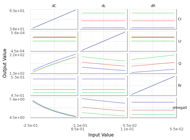
Construct a sinew plot to investigate how each input affects the outputs of the model. Answer the questions under observations below.

Note: You only need to sweep the random variables; you can use the nominal levels for the deterministic inputs.

(
    md_circuit

    >> gr.ev_sinews(df_det="nom")
    >> gr.pt_auto()
)

Calling plot_sinew_outputs....

/Users/zach/opt/anaconda3/envs/evc/lib/python3.9/site-packages/plotnine/utils.py:371: FutureWarning: The frame.append method is deprecated and will be removed from pandas in a future version. Use pandas.concat instead.

<ggplot: (8763303624807)>

Observations

• How does the hypothesis The variability in the resistance dR has no effect on the natural frequency omega0 hold up?

  • This hypothesis appears to be true! We see that the sweeps associated with omega0 and dR are completely flat, indicating that there is no effect of dR on omega0.