Grama: Fitting Multivariate Distributions

Purpose: As we’ve seen through studying a lot of datasets, many physical systems exhibit variability and other forms of uncertainty. Thus, it is beneficial to be able to model uncertainty using distributions. In the previous part of this exercise, we learned how to fit a distribution for a single quantity. Now we’ll learn how to deal with multiple related quantities.

In the final exercise e-grama08-duu we’ll see how to use a distribution model to do useful engineering work.

Setup

import grama as gr
DF = gr.Intention()
%matplotlib inline

For this exercise, we’ll study a dataset of observations on die cast aluminum parts.

from grama.data import df_shewhart

Dependency in the wild

We’ve seen lots of examples of dependency in datasets so far! Any case where we see “patterns” in a scatterplot are examples of some relationship (or dependency) between variables.

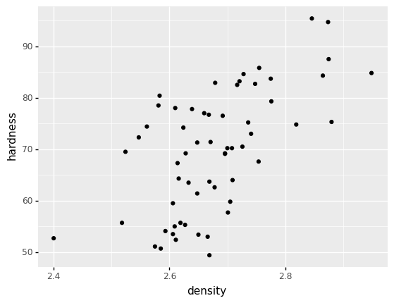
As a concrete example, let’s take a look at the measured density and hardness values from the cast aluminum dataset:

## NOTE: No need to edit
(
    df_shewhart
    >> gr.ggplot(gr.aes("density", "hardness"))
    + gr.geom_point()
)

<ggplot: (8744243135091)>

We can see a positive correlation between the two variables. If we wanted to model the density and hardness simultaneously, we would need to respect this dependency.

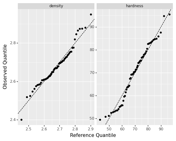
A normal distribution does a reasonable job representing both density and hardness separately.

## NOTE: No need to edit
(
    df_shewhart
    >> gr.tf_mutate(
        q_density=gr.qqvals(DF.density, "norm"),
        q_hardness=gr.qqvals(DF.hardness, "norm"),
    )
    >> gr.tf_rename(
        v_density="density",
        v_hardness="hardness",
    )
    >> gr.tf_pivot_longer(
        columns=["q_density", "q_hardness", "v_density", "v_hardness"],
        names_to=[".value", "var"],
        names_sep="_",
    )
    
    >> gr.ggplot(gr.aes("q", "v"))
    + gr.geom_abline(intercept=0, slope=1, linetype="dashed")
    + gr.geom_point()
    + gr.facet_wrap("var", scales="free")
    + gr.labs(x="Reference Quantile", y="Observed Quantile")
)

/home/zach/Git/py_grama/grama/tran_pivot.py:570: SettingWithCopyWarning: 
A value is trying to be set on a copy of a slice from a DataFrame

See the caveats in the documentation: https://pandas.pydata.org/pandas-docs/stable/user_guide/indexing.html#returning-a-view-versus-a-copy
/home/zach/Bin/anaconda3/envs/evc/lib/python3.9/site-packages/plotnine/facets/facet.py:487: FutureWarning: Passing a set as an indexer is deprecated and will raise in a future version. Use a list instead.
/home/zach/Bin/anaconda3/envs/evc/lib/python3.9/site-packages/plotnine/utils.py:371: FutureWarning: The frame.append method is deprecated and will be removed from pandas in a future version. Use pandas.concat instead.
/home/zach/Bin/anaconda3/envs/evc/lib/python3.9/site-packages/plotnine/utils.py:371: FutureWarning: The frame.append method is deprecated and will be removed from pandas in a future version. Use pandas.concat instead.
/home/zach/Bin/anaconda3/envs/evc/lib/python3.9/site-packages/plotnine/facets/facet.py:390: PlotnineWarning: If you need more space for the x-axis tick text use ... + theme(subplots_adjust={'wspace': 0.25}). Choose an appropriate value for 'wspace'.

<ggplot: (8744240703419)>

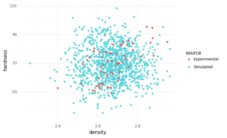
However, if we fit a normal for hardness and density separately, and ignore the dependency, we will end up with a model that does not respect the correlation we saw above:

## NOTE: No need to edit
# Build a model 
md_independence = (
    gr.Model("Independent Properties")
    >> gr.cp_marginals(
        density=gr.marg_fit("norm", df_shewhart.density),
        hardness=gr.marg_fit("norm", df_shewhart.hardness),
    )
    ## NOTE: This line is where things go wrong!
    # We can't just assume variables are independent
    # unless we have a good reason to do so.
    >> gr.cp_copula_independence()
)

# Draw simulated observations
(
    md_independence
    >> gr.ev_sample(n=1e3, df_det="nom", skip=True)
    >> gr.tf_mutate(source="Simulated")
    >> gr.tf_bind_rows(
        df_shewhart
        >> gr.tf_mutate(source="Experimental")
    )
    
    >> gr.ggplot(gr.aes("density", "hardness"))
    + gr.geom_point(gr.aes(color="source"))
    + gr.theme_minimal()
)

eval_sample() is rounding n...
Design runtime estimates unavailable; model has no timing data.

<ggplot: (8744240565745)>

Notice that this model does not respect the correlation we observe in the data. How can we fix this?

Marginal-Copula Approach

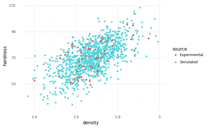
It turns out there is a drop-in solution for representing dependency; a copula is a mathematical tool to represent dependency between two (or more) random variables. We can fit a gaussian copula to represent the correlation we see between hardness and density.

## NOTE: No need to edit
# Build a model 
md_copula = (
    gr.Model("Independent Properties")
    >> gr.cp_marginals(
        density=gr.marg_fit("norm", df_shewhart.density),
        hardness=gr.marg_fit("norm", df_shewhart.hardness),
    )
    ## KEY DIFFERENCE: Fit a gaussian copula
    >> gr.cp_copula_gaussian(df_data=df_shewhart)
)

# Draw simulated observations
(
    md_copula
    >> gr.ev_sample(n=1e3, df_det="nom", skip=True)
    >> gr.tf_mutate(source="Simulated")
    >> gr.tf_bind_rows(
        df_shewhart
        >> gr.tf_mutate(source="Experimental")
    )
    
    >> gr.ggplot(gr.aes("density", "hardness"))
    + gr.geom_point(gr.aes(color="source"))
    + gr.theme_minimal()
)

eval_sample() is rounding n...
Design runtime estimates unavailable; model has no timing data.

<ggplot: (8744240524791)>

Note that this version of the model respects the correlation in the data!

Steps

When fitting a density for multiple uncertainties, we should follow an extended process:

1. Fit a marginal for each uncertain quantity

   • Follow the process from e-grama06-fit-univar; this should include checking for statistical control!

2. Fit a copula to relate the uncertain quantities

3. Assess the model

Case Study: Circuit Performance

To illustrate the full distribution-fitting process, we’ll work through a case study of circuit performance.

## NOTE: No need to edit
from grama.models import make_prlc_rand
md_circuit = make_prlc_rand()
md_circuit

/home/zach/Git/py_grama/grama/marginals.py:336: RuntimeWarning: divide by zero encountered in double_scalars

model: RLC with component tolerances

  inputs:
    var_det:
      L: [1e-09, 0.001]
      C: [0.001, 100]
      R: [0.001, 1.0]

    var_rand:
      dR: (+0) uniform, {'mean': '0.000e+00', 's.d.': '3.000e-02', 'COV': inf, 'skew.': 0.0, 'kurt.': 1.8}
      dL: (+0) uniform, {'mean': '0.000e+00', 's.d.': '6.000e-02', 'COV': inf, 'skew.': 0.0, 'kurt.': 1.8}
      dC: (+0) uniform, {'mean': '3.000e-01', 's.d.': '2.900e-01', 'COV': 0.96, 'skew.': 0.0, 'kurt.': 1.8}

    copula:
      Independence copula

  functions:
      f0: ['R', 'dR', 'L', 'dL', 'C', 'dC'] -> ['Rr', 'Lr', 'Cr']
      f1: ['Lr', 'Cr'] -> ['omega0']
      parallel RLC: ['omega0', 'Rr', 'Cr'] -> ['Q']

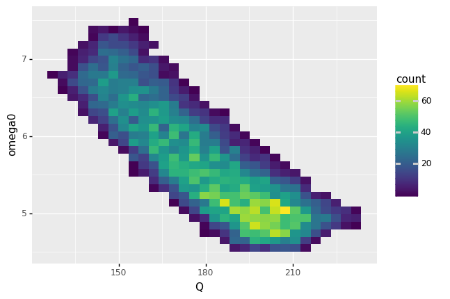
This circuit model has variability in its performance due to manufacturing variability. If we inspect its two outputs Q and omega0, we can see that they are quite variable, and exhibit a strong negative correlation.

## NOTE: No need to edit
df_circuit = (
    md_circuit
    >> gr.ev_sample(n=1e4, df_det="nom", seed=101)
)

(
    df_circuit
    >> gr.ggplot(gr.aes("Q", "omega0"))
    + gr.geom_bin2d()
)

eval_sample() is rounding n...

<ggplot: (8744240704705)>

Marginals

First, let’s fit distributions for the two quantities Q and omega0 separately.

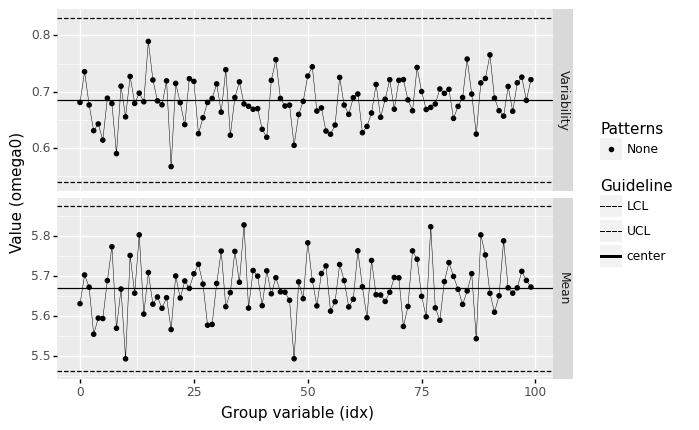
q1 Check for statistical control

Check for statistical control of the output omega0. Use a large batch size. Answer the questions under observations below.

## TASK: Make a control chart with a large batch size
(
    df_circuit
    >> gr.tf_mutate(idx=DF.index // 100)
    >> gr.pt_xbs(group="idx", var="omega0")
)

/home/zach/Git/py_grama/grama/tran_pivot.py:570: SettingWithCopyWarning: 
A value is trying to be set on a copy of a slice from a DataFrame

See the caveats in the documentation: https://pandas.pydata.org/pandas-docs/stable/user_guide/indexing.html#returning-a-view-versus-a-copy
/home/zach/Bin/anaconda3/envs/evc/lib/python3.9/site-packages/plotnine/utils.py:371: FutureWarning: The frame.append method is deprecated and will be removed from pandas in a future version. Use pandas.concat instead.
/home/zach/Bin/anaconda3/envs/evc/lib/python3.9/site-packages/plotnine/utils.py:371: FutureWarning: The frame.append method is deprecated and will be removed from pandas in a future version. Use pandas.concat instead.
/home/zach/Bin/anaconda3/envs/evc/lib/python3.9/site-packages/plotnine/utils.py:371: FutureWarning: The frame.append method is deprecated and will be removed from pandas in a future version. Use pandas.concat instead.

<ggplot: (8744243109816)>

Observations

• What batch size did you choose?

  • I chose a batch size of n_batch = 100.

• Does this process seem to be under statistical control?

  • Yes; there are not too many outlier batches, and there are no other suspicious patterns.

• Remind me: Is this quantity random? How do you know?

  • Yes! We generated these data as a random sample; they are random by-construction.

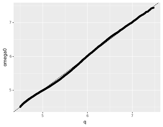
q2 Fit a marginal for omega0

Select a reasonable distribution for omega0 and fit it using the data df_circuit.omega0. Answer the questions under observations below.

## TASK: Fit a marginal for `omega0`

mg_omega0 = gr.marg_fit("beta", df_circuit.omega0)
## NOTE: Use the following to help check your work
(
    df_circuit
    >> gr.tf_mutate(q=gr.qqvals(DF.omega0, marg=mg_omega0))
    >> gr.ggplot(gr.aes("q", "omega0"))
    + gr.geom_abline(intercept=0, slope=1, linetype="dashed")
    + gr.geom_point()
)

<ggplot: (8744240478284)>

Observations

• How well does your distribution fit the data?

  • Quite well! There is some inaccuracy in the left tail, but overall it agrees nicely.

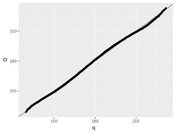
q3 Fit a marginal for Q

Select a reasonable distribution for Q and fit it using the data df_circuit.Q. Answer the questions under observations below.

## TASK: Fit a marginal for `Q`

mg_Q = gr.marg_fit("beta", df_circuit.Q)
## HINT: Use the assessment techniques discussed in 
# the previous exercise
(
    df_circuit
    >> gr.tf_mutate(q=gr.qqvals(DF.Q, marg=mg_Q))
    >> gr.ggplot(gr.aes("q", "Q"))
    + gr.geom_abline(intercept=0, slope=1, linetype="dashed")
    + gr.geom_point()
)
# solution-end

<ggplot: (8744240496150)>

Observations

• How well does your distribution fit the data?

  • Quite well! There is some wavering throughout, but the overall shape is correct.

Copula

Now that we’ve fit marginals for Q and omega0, we can work on representing their dependency.

The following code fits a model that neglects the dependency between Q and omega0. You will fit a gaussian copula and compare against this baseline model.

## NOTE: No need to edit
md_out_independence = (
    gr.Model("Circuit Output: Independence")
    >> gr.cp_marginals(
        omega0=mg_omega0,
        Q=mg_Q,
    )
    >> gr.cp_copula_independence()
)

md_out_independence 

model: Circuit Output: Independence

  inputs:
    var_det:

    var_rand:
      omega0: (+0) beta, {'mean': '5.680e+00', 's.d.': '6.700e-01', 'COV': 0.12, 'skew.': 0.34, 'kurt.': 2.27}
      Q: (+0) beta, {'mean': '1.793e+02', 's.d.': '2.142e+01', 'COV': 0.12, 'skew.': 0.05, 'kurt.': 2.25}

    copula:
      Independence copula

  functions:

q4 Fit a gaussian copula

Add a gaussian copula to the model md_out_copula.

Hint: The code above demonstrates how to add a gaussian copula to a grama model.

## TASK: Fit a gaussian copula model
md_out_copula = (
    gr.Model("Circuit Output: Copula")
    >> gr.cp_marginals(
        omega0=mg_omega0,
        Q=mg_Q,
    )
    >> gr.cp_copula_gaussian(df_data=df_circuit)
)

## NOTE: Do not edit; use this to check your work
assert \
    isinstance(md_out_copula.density.copula, gr.CopulaGaussian), \
    "md_out_copula must have a gaussian copula"

md_out_copula 

model: Circuit Output: Copula

  inputs:
    var_det:

    var_rand:
      omega0: (+0) beta, {'mean': '5.680e+00', 's.d.': '6.700e-01', 'COV': 0.12, 'skew.': 0.34, 'kurt.': 2.27}
      Q: (+0) beta, {'mean': '1.793e+02', 's.d.': '2.142e+01', 'COV': 0.12, 'skew.': 0.05, 'kurt.': 2.25}

    copula:
      Gaussian copula with correlations:
     var1 var2      corr
0  omega0    Q -0.817849

  functions:

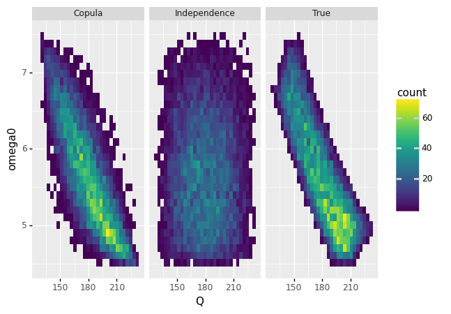
q5 Compare the models

Use the following code to compare the multivariate models; answer the questions under observations below.

## NOTE: No need to edit
(
    df_circuit
    >> gr.tf_mutate(source="True")
    >> gr.tf_bind_rows(
        md_out_independence
        >> gr.ev_sample(n=1e4, df_det="nom", skip=True)
        >> gr.tf_mutate(source="Independence")
    )
    >> gr.tf_bind_rows(
        md_out_copula
        >> gr.ev_sample(n=1e4, df_det="nom", skip=True)
        >> gr.tf_mutate(source="Copula")
    )
    
    >> gr.ggplot(gr.aes("Q", "omega0"))
    + gr.geom_bin2d()
    + gr.facet_wrap("source")
)

eval_sample() is rounding n...
Design runtime estimates unavailable; model has no timing data.
eval_sample() is rounding n...
Design runtime estimates unavailable; model has no timing data.

/home/zach/Bin/anaconda3/envs/evc/lib/python3.9/site-packages/plotnine/utils.py:371: FutureWarning: The frame.append method is deprecated and will be removed from pandas in a future version. Use pandas.concat instead.

<ggplot: (8744240495821)>

Observations

• How well does the independence model represent the true data?

  • Abysmal! The independence model does a terrible job representing the true data. For instance, the independence model does not capture the concentration of values at high Q and low omega0.

• What aspects does the copula model get correct?

  • The copula model gets the rough correlation correct, and correctly concentrates towards high Q and low omega0.

• What aspects does the copula model get incorrect?

  • The copula model “bows” along the edges, whereas the true data has a very “sharp” edge to the observations, almost like a bar.