Stats: Confidence Intervals and the CLT#
Purpose: When studying a limited dataset, we need a principled way to report our results with their uncertainties. Confidence intervals (CI) are an excellent way to summarize results, and the central limit theorem (CLT) helps us to construct these intervals. Eventually, we will use the same ideas underlying CI’s to detect patterns using statistical process monitoring.
Setup#
import grama as gr
DF = gr.Intention()
%matplotlib inline
Theory Fundamentals#
To make sense of confidence intervals, we will need a bit of background information. First up: Why are we studying confidence intervals?
Motivation: We might have seen other data#
Anytime we have a particular dataset, we should keep in mind that we might have seen other data.
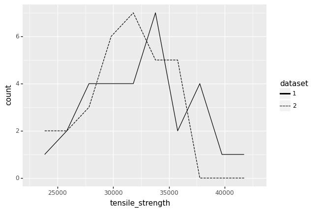
As a real example, let’s take a real dataset and split it in two. The following code loads a datset of tensile_strength values and splits the full dataset into two smaller datasets. We could have seen either of these two datasets, had we gathered half as many values.
from grama.data import df_shewhart

(
    df_shewhart
    >> gr.tf_mutate(dataset=DF.index % 2 + 1)
    >> gr.ggplot(gr.aes("tensile_strength"))
    + gr.geom_freqpoly(gr.aes(linetype="factor(dataset)"), bins=10)
    + gr.scale_linetype_discrete(name="dataset")
)
<ggplot: (8782076094004)>
We would draw different conclusions from these two different datasets. Dataset 1 has several observations with values over ~37,500 psi. However, Dataset 2 has no observations with values this large. In practice, we would have access to just one dataset; if we happened to have Dataset 2, we might assume that values of tensile_strength greater than 37,500 psi do not occur. Part of thinking statistically is keeping in mind possibilities like the one we see above: we might have seen other data.
To underscore this idea of limited data, let’s look at a simulated example. The following code defines a distribution with a specified mean.
## NOTE: No need to edit; run and inspect
# Define an uncertain quantity
mg_test = gr.marg_mom(
    "uniform",
    mean=0,
    sd=1,
)

mg_test
/Users/zach/Git/py_grama/grama/marginals.py:336: RuntimeWarning: divide by zero encountered in double_scalars
(+0) uniform, {'mean': '0.000e+00', 's.d.': '1.000e+00', 'COV': inf, 'skew.': 0.0, 'kurt.': 1.8}
From the marginal summary, we can see that the mean of the distribution is 0. However, if we have limited data then the mean of that sample will generally not be exactly zero:
## NOTE: No need to edit; run and inspect
# The true mean == 0; let's see what a limited sample gives
gr.mean(mg_test.r(10))
0.20323196014235362
Limited data leads to a form of error called sampling error. In practice we almost always have limited data, so sampling error is an unavoidable reality.
Sampling Distribution#
Let’s imagine for a moment that we did carry out data collection multiple times. Let’s illustrate this by splitting the tensile strength dataset into six separate subsets.
# Compute a set of estimates
(
    df_shewhart
    # Split into 6 groups
    >> gr.tf_mutate(dataset=DF.specimen % 6 + 1)
    # Compute the mean and variance over each sample
    >> gr.tf_group_by(DF.dataset)
    >> gr.tf_summarize(
        tys_mu=gr.mean(DF.tensile_strength),
        n=gr.n(DF.index),
    )
    >> gr.tf_ungroup()
)
| dataset | tys_mu | n | |
|---|---|---|---|
| 0 | 1 | 31936.6 | 10 |
| 1 | 2 | 30784.4 | 10 |
| 2 | 3 | 32413.4 | 10 |
| 3 | 4 | 35654.0 | 10 |
| 4 | 5 | 28975.0 | 10 |
| 5 | 6 | 31452.8 | 10 |
Note that the mean tys_mu is different for each of the datasets. This is an example of sampling error (also called sampling variability). Statisticians quantify sampling error by defining a population from which a smaller dataset is drawn. This smaller dataset is called a sample. In the tensile_strength case, the population is the infinite number of parts that could be manufactured according to the same process. Any time we make a finite number of parts (any real batch of parts!), we have a limited sample from the manufacturing process.
Sample vs Population
A population is the full set of values we are interested in. A sample is a small subset from that population. Since the sample is not the population, it has less information than the full population. A mismatch between information in the population and information in the sample (e.g., the population mean vs sample mean) is called sampling error.
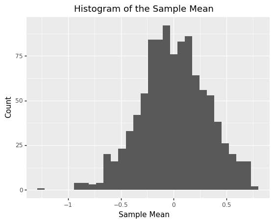
The sampling distribution is a conceptual tool used to quantify sampling variability in a chosen summary. Imagine that we repeatedly draw random samples (small datasets) of the same size from the target population. We then compute our chosen summary.
The following code defines a population mg_uniform, draws samples of size n=10, and computes the sample mean. The true mean is mean == 0; the variability we see around this value is sampling variability.
# Define a uniform distribution
# NOTE: The true mean is set here: `mean=0`
mg_uniform = gr.marg_mom("uniform", mean=0, sd=1)

# Simulated example
n = 10   # Sample size
m = 1000 # Number of samples

(
    # Generate m=1000 samples of size n=10
    gr.df_make(x=mg_uniform.r(n * m))
    >> gr.tf_mutate(group=DF.index % m)
    # Compute mean according to each sample
    >> gr.tf_group_by(DF.group)
    >> gr.tf_summarize(x_mean=gr.mean(DF.x))
    >> gr.tf_ungroup()
    # Visualize
    >> gr.ggplot(gr.aes("x_mean"))
    + gr.geom_histogram(bins=30)
    + gr.labs(
        x="Sample Mean",
        y="Count",
        title="Histogram of the Sample Mean",
    )
)
<ggplot: (8782076781294)>
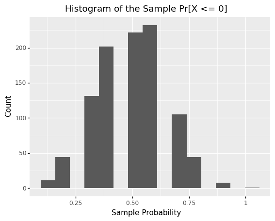
Sampling distributions are not limited to the mean! The following code defines the same population mg_uniform, the same sample size n=10, but computes the probability that X <= 0 rather than the mean. Note that the resulting sampling distribution looks quite different than the previous example.
# Define a uniform distribution
# NOTE: The true mean is set here: `mean=0`
mg_uniform = gr.marg_mom("uniform", mean=0, sd=1)

# Simulated example
n = 10   # Sample size
m = 1000 # Number of samples

(
    # Generate m=1000 samples of size n=10
    gr.df_make(x=mg_uniform.r(n * m))
    >> gr.tf_mutate(group=DF.index % m)
    # Compute mean according to each sample
    >> gr.tf_group_by(DF.group)
    >> gr.tf_summarize(pr_lo=gr.pr(DF.x <= 0))
    >> gr.tf_ungroup()
    # Visualize
    >> gr.ggplot(gr.aes("pr_lo"))
    + gr.geom_histogram(bins=15)
    + gr.labs(
        x="Sample Probability",
        y="Count",
        title="Histogram of the Sample Pr[X <= 0]",
    )
)
<ggplot: (8782076769856)>
The Sampling Distribution is based on Population, Sample Size, and Summary
The sampling distribution is a result of three ingredients: 1. The target population, 2. The chosen sample size, and 3. The chosen summary. The sampling distribution also assumes that each sample is drawn randomly from the population.
The sampling distribution is what we would observe under repeated data collection. However, gathering multiple datasets of the same size and computing independent summaries would be a highly inefficient way to use data! Instead, we can use the central limit theorem as a means to approximate a sampling distribution using just one dataset.
Central Limit Theorem (CLT)#
The central limit theorem (CLT) is most easily stated in terms of the sample mean. Let \(X \sim \rho\) be a random draw from a population with finite mean \(\mu\) and variance \(\sigma^2\). The sample mean is denoted \(\overline{X}_n\) and is defined as
Under independent, repeated observations from the same distribution \(X_i \sim \rho\), the central limit theorem states that \(\overline{X}_n\) becomes increasingly normal in its distribution as \(n\) is increased, regardless of the original distribution \(\rho\). That is
where \(\stackrel{d}{\to}\) means “convergence in distribution.” The CLT is useful because it gives us a way to quantify sampling error: Since the CLT holds regardless of where the data came from \(X \sim \rho\)—so long as \(|\mu| < \infty, \sigma < \infty\)—then we can characterize the sampling error in the sample mean \(\overline{X}_n\).
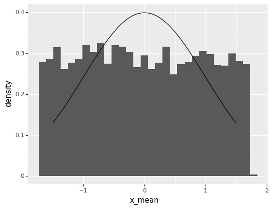
q1 Study CLT convergence behavior#
Adjust the sample size n below, run the code to inspect the results each time, then answer the questions under observations below.
## TODO: Adjust the sample size n
n = 1 # Sample size

## NOTE: No need to edit
# Draw a large sample
df_sample = gr.df_make(x=mg_test.r(5000))

(
    # Compute mean within each group
    df_sample
    >> gr.tf_mutate(i=DF.index // n)
    >> gr.tf_group_by(DF.i)
    >> gr.tf_summarize(
        x_mean=gr.mean(DF.x)
    )
    >> gr.tf_ungroup()

    # Visualize
    >> gr.ggplot(gr.aes("x_mean"))
    + gr.geom_histogram(gr.aes(y="stat(density)"), bins=30)
    + gr.geom_line(
        data=gr.df_make(x_mean=gr.linspace(-1.5, +1.5, 100))
        >> gr.tf_mutate(
            d=gr.marg_mom("norm", mean=0, sd=1/gr.sqrt(n)).d(DF.x_mean)
        ),
        mapping=gr.aes(y="d"),
    )
)
<ggplot: (8782085134111)>
Observations
Around what value of \(n\) does the histogram start to look like the normal distribution (black curve)?
Around values of \(n > 10\) the histogram starts to look like a normal distribution.
How does the “width” of the histogram change with \(n\)?
The “width” of the histogram tends to shrink with large \(n\), but it shrinks very slowly.
Confidence Intervals (CI)#
Since any estimated quantity has sampling error, it is common to report estimated values along with a confidence interval. A confidence interval (CI) is an expression of uncertainty; it will tend to be wider when the sampling error is larger. For the moment, let’s talk about how to compute a confidence interval; we’ll discuss how to interpret a confidence interval in a bit.
The CLT-based confidence interval for the mean is given by
where \(z_C\) is the relevant quantile of a standard normal distribution. This is based on capturing a specified fraction \(C\) of the distribution between the interval bounds. For instance, the following code computes \(z_C\) for \(C = 0.99\).
Terminology: Point Estimate vs Confidence Interval
A single value like a sample mean \(\overline{X}_n\) is called a point estimate, while a confidence interval is defined by two values (the interval endpoints).
## NOTE: No need to edit, this computes the relevant z_C value
C = 0.99 # 99% confidence level
mg_standard = gr.marg_mom("norm", mean=0, sd=1)
z_C = mg_standard.q(1 - (1 - C)/2)
print("z_C = {0:4.3f}".format(z_C))
z_C = 2.576
You can compute these CI bounds manually. However, the helper functions gr.mean_lo() and gr.mean_up() automate these calculations. For both functions, you can adjust the confidence level C with the alpha parameter.
q2 Compute a confidence interval#
Use the helper functions gr.mean_lo() and gr.mean_up() to compute confidence limits for the mean.
## TODO: Compute confidence limits for the mean;
df_ci = (
    gr.df_make(x=mg_test.r(10))
    >> gr.tf_summarize(
        x_lo=gr.mean_lo(DF.x),

        x_mean=gr.mean(DF.x),
        x_up=gr.mean_up(DF.x),

    )
)

## NOTE: Use this to check your work
assert \
    "x_lo" in df_ci.columns, \
    "You must compute x_lo"
assert \
    "x_up" in df_ci.columns, \
    "You must compute x_up"
assert \
    df_ci.x_lo[0] < df_ci.x_mean[0], \
    "x_lo should be smaller than x_mean"
assert \
    df_ci.x_mean[0] < df_ci.x_up[0], \
    "x_mean should be smaller than x_up"

df_ci
| x_lo | x_mean | x_up | |
|---|---|---|---|
| 0 | -0.540023 | 0.210576 | 0.961175 |
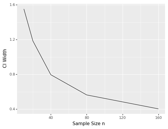
q3 Study the CI width#
The following code creates confidence intervals for samples of different sizes \(n\). Run the following code, inspect the results, and answer the questions under observations below.
## NOTE: No need to edit
df_sweep = gr.df_grid()
for i in [10, 20, 40, 80, 160]:
    df_sweep = (
        df_sweep
        >> gr.tf_bind_rows(
            gr.df_make(x=mg_test.r(i))
            >> gr.tf_summarize(
                x_lo=gr.mean_lo(DF.x),
                x_up=gr.mean_up(DF.x),
            )
            >> gr.tf_mutate(
                ci_width=DF.x_up - DF.x_lo,
                n=i,
            )
        )
    )

(
    df_sweep
    >> gr.ggplot(gr.aes("n", "ci_width"))
    + gr.geom_line()
    + gr.labs(
        x="Sample Size n",
        y="CI Width",
    )
)
<ggplot: (8782085128695)>
Observations
Compare the CI width behavior (figure immediately above) with the definition given earlier. What explains the curve above?
The CI expression contains a \(\sigma/\sqrt{n}\) term; the \(1/\sqrt{n}\) behavior is what we see above.
To halve the CI width, how would you need to change the sample size?
To halve the CI width, you would need to quadruple the sample size; note that the width goes as \(1/\sqrt{n}\), thus \(1/\sqrt{4n} = 1/(2\sqrt{n})\).
Interpreting Confidence Intervals#
Confidence intervals are constructed in a way that seeks to include the true value that we seek to estimate. However, the nature of uncertainty means we need to exercise care when interpreting a confidence interval.
Golden Rule of Confidence Intervals#
The “Golden Rule” for interpreting Confidence Intervals
When interpreting a confidence interval, we should assume the true value could be anywhere inside the interval.
Interpreting a CI as a range of possibilities helps us “hedge our bets”. The point estimate may suggest a favorable conclusion, but if the CI is wide, then an unfavorable conclusion may also be possible.
If a CI does not allow you to exclude an unfavorable possibility, it is an indication that you should gather another larger sample in order to study the same problem with greater statistical precision. You’ll practice these ideas in the following exercises.
Confidence in procedure, not in the interval
A subtle point about confidence intervals is that our confidence is in the long-run properties of constructing many intervals, not in any single interval. Any individual interval either does or does not include its true value: the “probability” for a single interval is either 0 or 1.
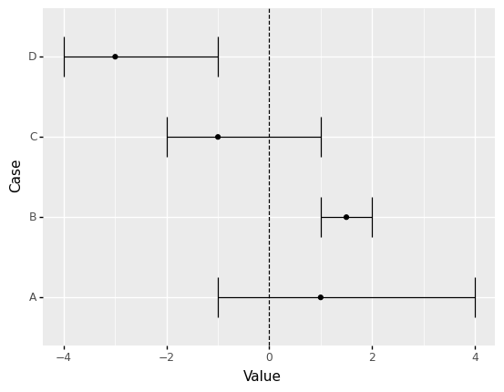
q4 Interpret these intervals#
Study the following intervals, answer the questions under observations below.
## NOTE: No need to edit; run and inspect
(
    gr.df_make(
        case=["A", "B", "C", "D"],
        x_lo=[ -1,   1,  -2,  -4],
        x_mu=[  1, 1.5,  -1,  -3],
        x_up=[  4,   2,   1,  -1],
    )
    >> gr.ggplot(gr.aes("case"))
    + gr.geom_errorbar(gr.aes(ymin="x_lo", ymax="x_up"))
    + gr.geom_point(gr.aes(y="x_mu"))
    + gr.geom_hline(yintercept=0, linetype="dashed")
    + gr.coord_flip()
    + gr.labs(
        y="Value",
        x="Case",
    )
)
<ggplot: (8782105817853)>
Observations
Is Case A greater than zero?
Unclear; the confidence interval includes zero, so A could very well be negative.
Is Case B greater than zero?
Most likely yes; the entire confidence interval is greater than zero.
Is Case C less than zero?
Unclear; the confidence interval includes zero, so C could very well be positive.
Is Case D less than zero?
Most likely yes; the entire confidence interval is less than zero.
Probability Estimation#
Remember that we learned in the previous exercise stat04-distributions that probability can be expressed as a mean (expectation). Thus, we can apply the same ideas about confidence intervals when estimating probabilities.
To demonstrate, let’s study a simple structural model.
from grama.models import make_cantilever_beam
md_beam = make_cantilever_beam()
md_beam
model: Cantilever Beam

  inputs:
    var_det:
      t: [2, 4]
      w: [2, 4]

    var_rand:
      H: (+1) norm, {'mean': '5.000e+02', 's.d.': '1.000e+02', 'COV': 0.2, 'skew.': 0.0, 'kurt.': 3.0}
      V: (+1) norm, {'mean': '1.000e+03', 's.d.': '1.000e+02', 'COV': 0.1, 'skew.': 0.0, 'kurt.': 3.0}
      E: (+0) norm, {'mean': '2.900e+07', 's.d.': '1.450e+06', 'COV': 0.05, 'skew.': 0.0, 'kurt.': 3.0}
      Y: (-1) norm, {'mean': '4.000e+04', 's.d.': '2.000e+03', 'COV': 0.05, 'skew.': 0.0, 'kurt.': 3.0}

    copula:
      Independence copula

  functions:
      cross-sectional area: ['w', 't'] -> ['c_area']
      limit state: stress: ['w', 't', 'H', 'V', 'E', 'Y'] -> ['g_stress']
      limit state: displacement: ['w', 't', 'H', 'V', 'E', 'Y'] -> ['g_disp']
This model has two outputs that model failure modes: g_stress <= 0 when the beam exceeds its maximum stress, and g_disp <= 0 when the tip deflection is beyond its designed limit. We can assess the probability of failure for both failure modes:
# NOTE: No need to edit
(
    md_beam
    >> gr.ev_sample(n=100, df_det="nom")
    >> gr.tf_summarize(
        pof_stress=gr.pr(DF.g_stress <= 0),
        pof_disp=gr.pr(DF.g_disp <= 0),
    )
)
| pof_stress | pof_disp | |
|---|---|---|
| 0 | 0.06 | 0.06 |
Like the mean CI helpers, grama provides gr.pr_lo() and gr.pr_up() to easily compute confidence intervals on a probability:
The probability CI helpers are different
Note that the probability CI helpers gr.pr_lo() and gr.pr_up() are different from gr.mean_lo() and gr.mean_up(); namely, they only return values between [0, 1]. Make sure to only use the probability helpers when estimating probabilities!
## NOTE: No need to edit; run and inspect
(
    md_beam
    >> gr.ev_sample(n=100, df_det="nom", seed=101)
    >> gr.tf_summarize(
        pof_lo=gr.pr_lo(DF.g_stress <= 0),
        pof=gr.pr(DF.g_stress <= 0),
        pof_up=gr.pr_up(DF.g_stress <= 0),
    )
)
| pof_lo | pof | pof_up | |
|---|---|---|---|
| 0 | 0.003477 | 0.02 | 0.106641 |
This is an extremely wide confidence interval for the probability of failure; I get a value of pof anywhere between 0.003 and 0.11!
q5 Adjust the sample size#
Adjust the sample size n to achieve a CI width less than 0.1. Answer the questions under observations below.
## TODO: Adjust the sample size
df_pof = (
    md_beam
    >> gr.ev_sample(

        n=5e4,
        df_det="nom",
    )
    >> gr.tf_summarize(
        pof_lo=gr.pr_lo(DF.g_stress <= 0),
        pof=gr.pr(DF.g_stress <= 0),
        pof_up=gr.pr_up(DF.g_stress <= 0),
    )
)

## NOTE: No need to edit; use to check your work
assert \
    abs(df_pof.pof_up[0] - df_pof.pof_lo[0]) < 0.1, \
    "CI is too wide; increase `n`"

df_pof
eval_sample() is rounding n...
| pof_lo | pof | pof_up | |
|---|---|---|---|
| 0 | 0.033094 | 0.03534 | 0.037732 |
Observations
Is the
pofsmaller than0.04?At a sample size of
n=5e4I find thatpof_up ~ 0.03973, which suggests thatpof < 0.04. At a sample size ofn=20(as given in the default), the upper confidence limitpof_upexceeds0.04, so we need to increasenin order to make this determination.
q6 Design for small failure rate#
Adjust the deterministic variables w and t in order to confidently achieve a probability of failure due to stress less than 0.001.
Hint: You adjusted the sample size n in the previous exercise. Make sure to use that learning when tackling this exercise.
## TODO: Adjust the deterministic variables `w, t` to achieve a probability
## of failure less than 0.001
df_pof_small = (
    md_beam
    >> gr.ev_sample(

        n=1e4, # A larger sample size is necessary for a small CI
        df_det=gr.df_make(w=3.0, t=3.5),
    )
    >> gr.tf_summarize(
        pof_lo=gr.pr_lo(DF.g_stress <= 0),
        pof=gr.pr(DF.g_stress <= 0),       # I find that pof ~= 0.0
        pof_up=gr.pr_up(DF.g_stress <= 0), # pof_up must be < 0.001
    )
)

## NOTE: Use this to check your work
print(df_pof_small)

assert \
    df_pof_small.pof_up.values[0] < 0.001, \
    "The upper CI bound for the POF is not less than 0.001"
eval_sample() is rounding n...
         pof_lo  pof    pof_up
0  5.421011e-20  0.0  0.000787
Real vs Error#
In stat02-source we learned that we should treat real and erroneous sources of variability differently. Let’s apply that thinking to the beam example.
q7 Selecting the proper statistical technique#
Suppose the variability exhibited by the model md_beam is real. Study the results from the simulation below, and answer the questions under observations below.
## TODO: No need to edit; run and inspect the results
(
    md_beam
    >> gr.ev_sample(
        n=1e4,
        df_det="nom",
    )
    >> gr.tf_summarize(
        g_lo=gr.mean_lo(DF.g_stress),
        g_mean=gr.mean(DF.g_stress),
        g_up=gr.mean_up(DF.g_stress),

        pof_lo=gr.pr_lo(DF.g_stress <= 0),
        pof=gr.pr(DF.g_stress <= 0),
        pof_up=gr.pr_up(DF.g_stress <= 0),
    )
)
eval_sample() is rounding n...
| g_lo | g_mean | g_up | pof_lo | pof | pof_up | |
|---|---|---|---|---|---|---|
| 0 | 0.165897 | 0.168285 | 0.170674 | 0.032335 | 0.0373 | 0.042994 |
Observations
Is the variability in
g_stressreal or erroneous?We’re assuming that the variability exhibited by this model is real, so the variability in
g_stressis real.
Is the mean of
g_stressgreater than zero?Yes; the confidence interval for
g_stressis entirely above zero (0 < g_lo).
What is the probability of failure due to stress?
The probability of failure is between
[0.03, 0.04]; it is fairly small but non-negligible.
Which of the two statistical techniques—computing the mean or computing a probability of failure—better characterizes the safety of this system? Why?
The probability of failure better characterizes the safety of the system. Remember that the mean is most appropriate when variability is purely error, so it is an inappropriate summary of the behavior of this system. A probability of failure is a very natural measure of safety.