Demo Notebook 2022-07-11

Demos from the live sessions on 2022-07-11.

Setup

import grama as gr
import pandas as pd
import numpy as np
DF = gr.Intention()
%matplotlib inline

# NOTE: No need to edit; load the archival data
filename_archival = "../challenges/data/doe-wide.csv"
df_archival = pd.read_csv(filename_archival)
df_archival.head()

	d	n	f_com	H	W	M_max	mass	dMdtheta_avs	dMdtheta_0	M_min	BM	angle	int_M_stable	GM
0	0.414694	0.969522	0.384112	1.931260	1.390651	5.004726e-16	0.019592	NaN	-1.459991	-4.952630	0.108234	NaN	-8.019885	0.193949
1	0.242507	1.195436	0.656740	2.713299	3.580954	7.277457e+00	0.046730	NaN	9.916728	-5.402567	0.425216	NaN	3.675911	-0.557773
2	0.441223	0.936345	0.672138	1.446188	3.744617	6.550768e+00	0.040910	8.237037	-11.668754	-5.879390	1.073773	1.617128	-5.681558	0.768485
3	0.689483	0.882652	0.648739	1.210221	2.530339	1.149756e+00	0.034526	2.380926	-8.409095	-2.228434	0.764303	1.509121	-2.070254	0.652657
4	0.497305	0.780804	0.235978	2.502149	1.505777	7.886234e-16	0.029039	NaN	-8.644337	-14.019720	0.103794	NaN	-25.533024	0.796536

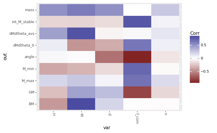
Correlation tile plot

Since there are NaN values in our dataset df_archival, we need to handle them somehow. We can use the nan_drop=True option in gr.tf_iocorr() to simply drop the NaN’s when computing correlations.

var = ["d", "n", "f_com", "H", "W"]
out = [
    "M_max", 
    "M_min", 
    "mass", 
    "dMdtheta_avs", 
    "dMdtheta_0", 
    "BM", 
    "GM",
    "angle",
    "int_M_stable",
]

(
    df_archival
    >> gr.tf_iocorr(
        var=var, 
        out=out, 
        nan_drop=True,
    )
    >> gr.pt_auto()
)

Calling plot_corrtile....

<ggplot: (8760894671336)>

From this plot, we can see that the correlation between H and dMdtheta_0 is small, as is the correlation between n and dMdtheta_0. This suggests that the linear relationship between the two is quite small. But keep in mind that a nonlinear relationship could also exist.

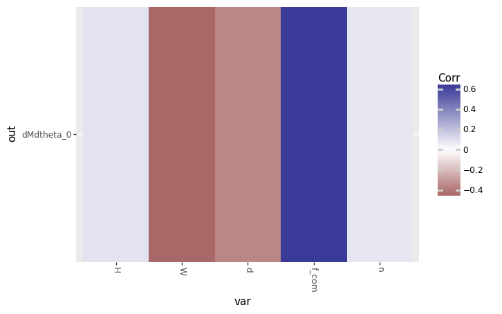
We can also trim the out argument to produce a more focused plot:

(
    df_archival
    >> gr.tf_iocorr(
        var=var, 
        out=["dMdtheta_0"],
        nan_drop=True,
    )
    >> gr.pt_auto()
)

Calling plot_corrtile....

<ggplot: (8760914488950)>

A plot like this looks somewhat strange. Really, we only have five numbers, so we might as well just look at the table of values:

(
    df_archival
    >> gr.tf_iocorr(
        var=var, 
        out=["dMdtheta_0"],
        nan_drop=True,
    )
    >> gr.tf_arrange(DF.rho)
)

	rho	var	out
0	-0.424045	W	dMdtheta_0
1	-0.336092	d	dMdtheta_0
2	0.074710	n	dMdtheta_0
3	0.089236	H	dMdtheta_0
4	0.611931	f_com	dMdtheta_0

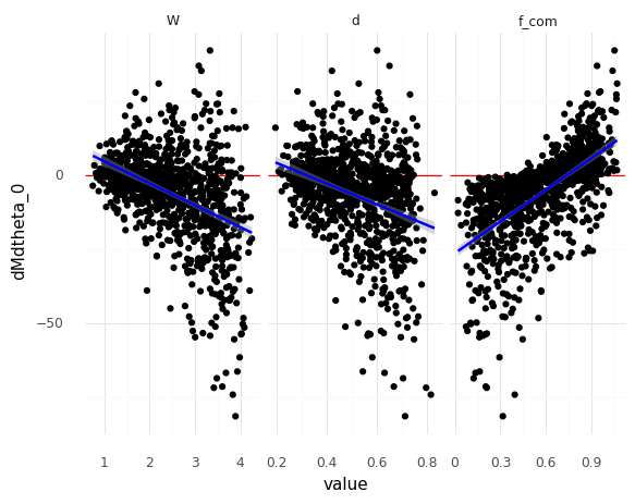
Detailed Scatterplot

Here’s how I incorporate multiple scatterplots into a single figure. Pivoting the data allows me to use faceting.

(
    df_archival
    >> gr.tf_select(
        "dMdtheta_0",
        "W",
        "d",
        "f_com"
    )
    >> gr.tf_pivot_longer(
        columns=["W", "d", "f_com"],
        names_to="var",
        values_to="value",
    )
    
    >> gr.ggplot(gr.aes("value", "dMdtheta_0"))
    + gr.geom_hline(yintercept=0, color="red")
    + gr.geom_point()
    + gr.geom_smooth(color="blue")
    + gr.facet_grid("~var", scales="free_x")
    + gr.theme_minimal()
)

<ggplot: (8760835732209)>

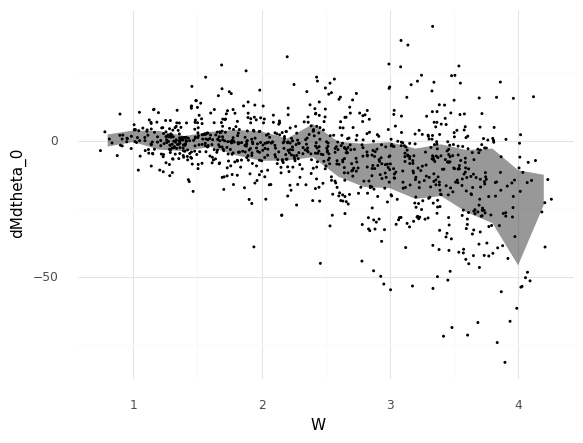
Plotting quantiles

factor = 1/2
(
    df_archival
    
    >> gr.ggplot(gr.aes("W", "dMdtheta_0"))
    + gr.geom_ribbon(
        data=df_archival
        >> gr.tf_mutate(W_bin=gr.round(DF.W*factor, decimals=1)/factor)
        >> gr.tf_group_by(DF.W_bin)
        >> gr.tf_summarize(
            ymin=gr.quant(DF.dMdtheta_0, 0.25),
            dMdtheta_0=gr.mean(DF.dMdtheta_0),
            ymax=gr.quant(DF.dMdtheta_0, 0.75),
        ),
        mapping=gr.aes(x="W_bin", ymin="ymin", ymax="ymax"),
        alpha=2/4,
    )
    + gr.geom_point(size=0.2)
    + gr.theme_minimal()
)

<ggplot: (8760881143866)>

Targeted Sinew Plot

Note that gr.pt_auto() calls other plotting functions with default arguments. We can call the same function with different arguments to tweak a visual. For instance, we can plot a smaller number of outputs for a more focused plot:

## Targeting a single output
(
    df_sinews
    >> gr.pt_sinew_outputs(
        var=["W", "H", "d", "f_com", "n"],
        out=["dMdtheta_0"],
    )
)

## Targeting a couple inputs
(
    df_sinews
    >> gr.pt_sinew_outputs(
        var=["d", "f_com"],
        out=["dMdtheta_0"],
    )
)

## Manually constructing a single sweep (over W)
(
    df_sinews
    >> gr.tf_filter(DF.sweep_var == "W")
    
    >> gr.ggplot(gr.aes("W", "dMdtheta_0"))
    + gr.geom_line(gr.aes(color="factor(sweep_ind)"))
)