Data: Joining Datasets#

Purpose: Often our data are scattered across multiple sets. In this case, we need to be able to join data.

Setup#

import grama as gr
DF = gr.Intention()
%matplotlib inline

Danger! Naive “binding” of data#

The simplest means we have to combine two datasets is to bind them together. The verb gr.tf_bind_rows() binds together two datasets vertically (adds rows to rows), while gr.tf_bind_cols() binds two datasets horizontally (adds new columns to the dataset). These are very simple ways to combine datasets; for example:

## NOTE: No need to edit
(
    gr.df_make(numbers=[1,2,3,4])
    >> gr.tf_bind_cols(
        gr.df_make(letters=["A", "B", "C", "D"])
    )
)

	numbers	letters
0	1	A
1	2	B
2	3	C
3	4	D

Binding is appropriate when we have strong knowledge of how our data are structured; we blindly smash together rows or columns to make a new dataframe, so we’d better be sure those rows/columns are in the right order! Otherwise, we may get surprising (and wrong) results….

q1 What went wrong with this bind?#

Run the following code and answer the questions under observations below.

Hint: If you’re not a Beatles fan, it may be helpful to consult the relevant personnel page on Wikipedia.

## NOTE: No need to edit; run and inspect
# Setup
df_beatles = gr.df_make(
    band=["Beatles"] * 4,
    name=["John", "Paul", "George", "Ringo"],
)

df_beatles_instruments = gr.df_make(
    surname=["McCartney", "Harrison", "Starr", "Lennon"],
    instrument=["bass", "guitar", "drums", "guitar"]
)

# Attempt to combine the datasets... to disastrous results!
(
    df_beatles
    >> gr.tf_bind_cols(df_beatles_instruments)
)

	band	name	surname	instrument
0	Beatles	John	McCartney	bass
1	Beatles	Paul	Harrison	guitar
2	Beatles	George	Starr	drums
3	Beatles	Ringo	Lennon	guitar

Observations

What went wrong in binding df_beatles and df_beatles_instruments?
- The rows of df_beatles were not in the same order as the rows of df_beatles_instruments! Now we have absurd combinations such as "Ringo Lennon" and "George Starr".

A safer way: “Joining” datasets#

A safer way to combine two datasets is to not assume they are ordered correctly. Instead, we can use common information to join two datasets. In order to do a join, we must have a set of “keys” by which to combine data from the two datasets. For instance, if we had a DataFrame with both name and surname, we could join to df_beatles1 by the name column.

## NOTE: No need to edit
df_beatles_surnames = gr.df_make(
    name=["John", "Paul", "George", "Ringo"],
    surname=["Lennon", "McCartney", "Harrison", "Starr"],
)

df_beatles_names = (
    df_beatles
    >> gr.tf_left_join(df_beatles_surnames, by="name")
)
df_beatles_names

	band	name	surname
0	Beatles	John	Lennon
1	Beatles	Paul	McCartney
2	Beatles	George	Harrison
3	Beatles	Ringo	Starr

Note that this correctly associates names with surnames.

q2 Do a join#

Use gr.tf_left_join() to associate each instrument with the correct band member.

## TASK: Join df_beatles2 correctly to add the `instrument` column
df_beatles_full = (
    df_beatles_names
    >> gr.tf_left_join(
        df_beatles_instruments,
        by="surname",
    )
)

## NOTE: Use this to check your work
assert \
    "instrument" in df_beatles_full.columns, \
    "df_beatles_full does not have an `instrument` column"

assert \
    df_beatles_full[df_beatles_full.name == "Ringo"].instrument.values[0] == "drums", \
    "Ringo Starr played drums!"

df_beatles_full

	band	name	surname	instrument
0	Beatles	John	Lennon	guitar
1	Beatles	Paul	McCartney	bass
2	Beatles	George	Harrison	guitar
3	Beatles	Ringo	Starr	drums

There’s a very important lesson here: In general, don’t trust gr.tf_bind_cols. It’s easy in the example above to tell there’s a problem because the data are small; when working with larger datasets, the software will happily give you the wrong answer if you give it the wrong instructions. Whenever possible, use some form of join to combine datasets.

Types of joins#

There are several types of joins:

Name	Type	Description
`gr.tf_left_join()`	Mutating join	Preserves rows in the left DataFrame being joined
`gr.tf_right_join()`	Mutating join	Preserves rows in the right DataFrame being joined
`gr.tf_inner_join()`	Mutating join	Preserves rows common to both DataFrames being joined
`gr.tf_outer_join()`	Mutating join	Preserves all rows in both DataFrames being joined
`gr.tf_semi_join()`	Filtering join	Returns all rows in left DataFrame that have a match in the right DataFrame
`gr.tf_anti_join()`	Filtering join	Returns all rows in left DataFrame that have no match in the right DataFrame

We’ll discuss (and use!) each of these below.

Mutating joins#

A mutating join is a join that also performs a mutation—it adds columns to the DataFrame. Like we saw above, we can use a mutating join to add information to a datset. However, there are four different types of mutating

## NOTE: No need to edit
df_beatles_names = gr.df_make(
    name=["John", "Paul", "George", "Ringo", "George"],
    surname=["Lennon", "McCartney", "Harrison", "Starr", "Martin"],
)

df_beatles_roles = gr.df_make(
    surname=["Lennon", "McCartney", "Harrison", "Starr", "Epstein"],
    role=["Bandmate", "Bandmate", "Bandmate", "Bandmate", "Manager"],
)

You’ll investigate how the various join types function in the next task:

q3 Test the joins#

Uncomment one line at a time and run the code below. Answer the questions under observations below.

## TASK: Uncomment one line at a time and run; document your findings
(
    df_beatles_names
    >> gr.tf_left_join(df_beatles_roles, by="surname")
    # >> gr.tf_right_join(df_beatles_roles, by="surname")
    # >> gr.tf_inner_join(df_beatles_roles, by="surname")
    # >> gr.tf_outer_join(df_beatles_roles, by="surname")
)

	name	surname	role
0	John	Lennon	Bandmate
1	Paul	McCartney	Bandmate
2	George	Harrison	Bandmate
3	Ringo	Starr	Bandmate
4	George	Martin	NaN

Observations

Which rows does tf_left_join() preserve?
- This preserves the rows in the left (first) DataFrame.
Which rows does tf_right_join() preserve?
- This preserves the rows in the right (second) DataFrame.
Which rows does tf_inner_join() preserve?
- This preserves the rows common to both DataFrames.
Which rows does tf_outer_join() preserve?
- This preserves all rows in both DataFrames.

Visual Aid: Types of Joins#

The following visual may help you make sense of the four mutating joins; it depicts the four verbs as Venn diagrams for the left (L) and right (R) DataFrames in the join.

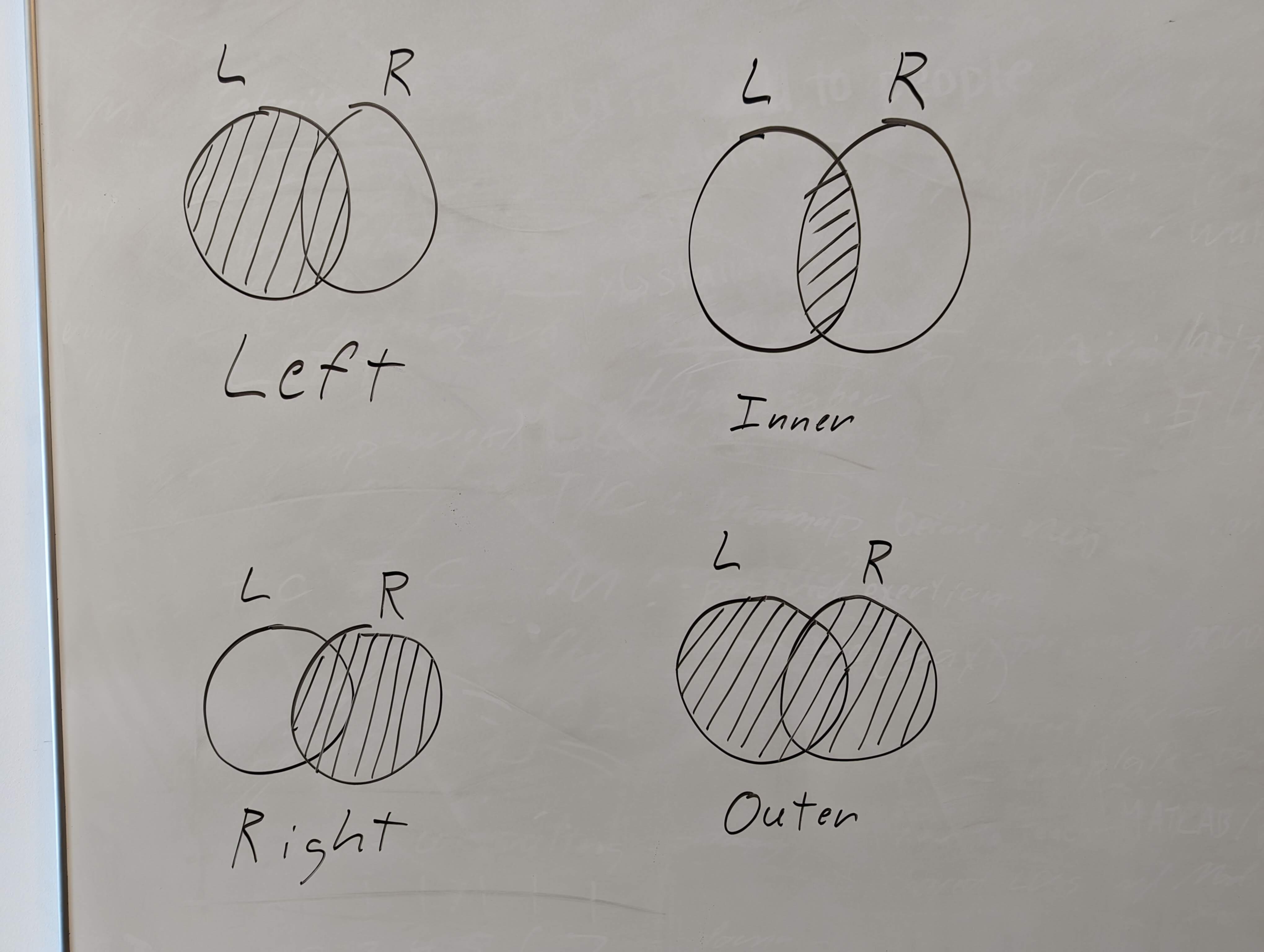
Venn diagrams for four types of joins: left, right, inner, outer

You may also find this image helpful for visualizing the join types.

Danger! Non-unique keys#

Note that when we do any sort of join, we need unique keys. We’ll run into trouble if the provided keys do not uniquely identify each row. For example, Harrison and Martin share a given name:

## NOTE: No need to edit
df_beatles_names

	name	surname
0	John	Lennon
1	Paul	McCartney
2	George	Harrison
3	Ringo	Starr
4	George	Martin

Look at what happens when we join on first name only:

## NOTE: No need to edit; this gives incorrect results due to non-unique keys
(
    df_beatles_names
    >> gr.tf_full_join(
        gr.df_make(
            name=["Paul", "George", "Ringo", "John"],
            instrument=["bass", "guitar", "drums", "guitar"]
        ),
        by="name"
    )
)

	name	surname	instrument
0	John	Lennon	guitar
1	Paul	McCartney	bass
2	George	Harrison	guitar
3	George	Martin	guitar
4	Ringo	Starr	drums

George Martin didn’t play the guitar in the Beatles! He was their producer.

If a single key is not unique, we can use multiple keys for the join:

## NOTE: No need to edit; using multiple keys corrects the issue
(
    df_beatles_names
    >> gr.tf_full_join(
        gr.df_make(
            name=["Paul", "George", "Ringo", "John"],
            surname=["McCartney", "Harrison", "Starr", "Lennon"],
            instrument=["bass", "guitar", "drums", "guitar"]
        ),
        by=["name", "surname"],
    )
)

	name	surname	instrument
0	John	Lennon	guitar
1	Paul	McCartney	bass
2	George	Harrison	guitar
3	Ringo	Starr	drums
4	George	Martin	NaN

Filtering joins#

Mutating joins add new columns, but filtering joins simply filter the DataFrame. A filter join is particularly helpful when a filter is difficult to express in gr.tf_filter(), but easy to express as a set of keys (perhaps with multiple key columns).

As a first example, we can filter on all of the "George"’s with a gr.tf_semi_join().

## NOTE: No need to edit
(
    df_beatles_names
    >> gr.tf_semi_join(
        gr.df_make(name=["George"]),
        by="name",
    )
)

	name	surname
0	George	Harrison
1	George	Martin

As we saw before, a single key will often not be enough to uniquely identify a row. For instance, the following will filter down to a numer of non-Beatle players:

## NOTE: No need to edit
(
    gr.df_make(
        surname=["Clapton", "Harrison", "Shankar", "Wooten", "McCartney"],
        instrument=["guitar", "guitar", "sitar", "bass", "bass"],
    )
    >> gr.tf_semi_join(
        df_beatles_instruments,
        by="instrument"
    )
)

	surname	instrument
0	Clapton	guitar
1	Harrison	guitar
2	Wooten	bass
3	McCartney	bass

q4 Semi-join with multiple keys#

Construct the by argument for gr.tf_semi_join() below to filter to only persons who were in the Beatles.

## TASK: Construct the `by` argument below to filter to *only* persons who were in the Beatles
(
    gr.df_make(
        surname=["Clapton", "Harrison", "Shankar", "Wooten", "McCartney"],
        instrument=["guitar", "guitar", "sitar", "bass", "bass"],
    )
    >> gr.tf_semi_join(
        df_beatles_instruments,

        by=["instrument", "surname"]
    )
)

	surname	instrument
0	Harrison	guitar
1	McCartney	bass

Going Further: Airports dataset#

We’ll use the nycflights13 package to demonstrate joins in a more realistic situation. This is a dataset of flights involving the New York City area during 2013.

from nycflights13 import flights as df_flights
df_flights

	year	month	day	dep_time	sched_dep_time	dep_delay	arr_time	sched_arr_time	arr_delay	carrier	flight	tailnum	origin	dest	air_time	distance	hour	minute	time_hour
0	2013	1	1	517.0	515	2.0	830.0	819	11.0	UA	1545	N14228	EWR	IAH	227.0	1400	5	15	2013-01-01T10:00:00Z
1	2013	1	1	533.0	529	4.0	850.0	830	20.0	UA	1714	N24211	LGA	IAH	227.0	1416	5	29	2013-01-01T10:00:00Z
2	2013	1	1	542.0	540	2.0	923.0	850	33.0	AA	1141	N619AA	JFK	MIA	160.0	1089	5	40	2013-01-01T10:00:00Z
3	2013	1	1	544.0	545	-1.0	1004.0	1022	-18.0	B6	725	N804JB	JFK	BQN	183.0	1576	5	45	2013-01-01T10:00:00Z
4	2013	1	1	554.0	600	-6.0	812.0	837	-25.0	DL	461	N668DN	LGA	ATL	116.0	762	6	0	2013-01-01T11:00:00Z
...	...	...	...	...	...	...	...	...	...	...	...	...	...	...	...	...	...	...	...
336771	2013	9	30	NaN	1455	NaN	NaN	1634	NaN	9E	3393	NaN	JFK	DCA	NaN	213	14	55	2013-09-30T18:00:00Z
336772	2013	9	30	NaN	2200	NaN	NaN	2312	NaN	9E	3525	NaN	LGA	SYR	NaN	198	22	0	2013-10-01T02:00:00Z
336773	2013	9	30	NaN	1210	NaN	NaN	1330	NaN	MQ	3461	N535MQ	LGA	BNA	NaN	764	12	10	2013-09-30T16:00:00Z
336774	2013	9	30	NaN	1159	NaN	NaN	1344	NaN	MQ	3572	N511MQ	LGA	CLE	NaN	419	11	59	2013-09-30T15:00:00Z
336775	2013	9	30	NaN	840	NaN	NaN	1020	NaN	MQ	3531	N839MQ	LGA	RDU	NaN	431	8	40	2013-09-30T12:00:00Z

336776 rows × 19 columns

q5 Make a “grid” of filter criteria#

Use gr.df_grid() to make a DataFrame with the rows.

`month`	`dest`
8	“SJC”
8	“SFO”
8	“OAK”
9	“SJC”
9	“SFO”
9	“OAK”

Note: We’ll use this grid soon in a filtering join.

## TASK: Use gr.df_grid() to make the DataFrame described above

df_criteria = gr.df_grid(
    month=[8, 9],
    dest=["SJC", "SFO", "OAK"]
)
## NOTE: Use this to check your work
assert \
    "month" in df_criteria.columns, \
    "df_criteria does not have a 'month' column"

assert \
    "dest" in df_criteria.columns, \
    "df_criteria does not have a 'dest' column"

assert \
    df_criteria.shape[0] == 6, \
    "df_criteria has the wrong number of columns"

df_criteria

	month	dest
0	8	SJC
1	9	SJC
2	8	SFO
3	9	SFO
4	8	OAK
5	9	OAK

There are many carriers in this dataset; let’s figure out which carriers are associated with flights in August (month==8) and September (month==9) to the San Francisco Bay Area (SJC, SFO, OAK).

(
    df_flights
    >> gr.tf_count(DF.carrier)
)

	carrier	n
0	9E	18460
1	AA	32729
2	AS	714
3	B6	54635
4	DL	48110
5	EV	54173
6	F9	685
7	FL	3260
8	HA	342
9	MQ	26397
10	OO	32
11	UA	58665
12	US	20536
13	VX	5162
14	WN	12275
15	YV	601

q6 Count the Bay area carriers#

Perform a semi-join to filter df_flights using all the columns of df_criteria. Answer the questions under observations below.

## TASK: Semi-join with df_criteria
(
    df_flights

    >> gr.tf_semi_join(df_criteria, by=["month", "dest"])
    >> gr.tf_count(DF.carrier)
)

	carrier	n
0	AA	239
1	B6	306
2	DL	324
3	UA	1305
4	VX	410

Observations

How many carriers provided flights to the SF Bay Area in the months considered?
- There are 5 such carriers
How does this number of carriers compare with the total number of carriers?
- This is considerably fewer carriers!

Unless you work in the airline industry, it’s probably difficult to make sense of these carrier codes. Thankfully the nycflights13 package comes with a dataset that helps disambiguate these codes:

from nycflights13 import airlines as df_airlines
df_airlines

	carrier	name
0	9E	Endeavor Air Inc.
1	AA	American Airlines Inc.
2	AS	Alaska Airlines Inc.
3	B6	JetBlue Airways
4	DL	Delta Air Lines Inc.
5	EV	ExpressJet Airlines Inc.
6	F9	Frontier Airlines Inc.
7	FL	AirTran Airways Corporation
8	HA	Hawaiian Airlines Inc.
9	MQ	Envoy Air
10	OO	SkyWest Airlines Inc.
11	UA	United Air Lines Inc.
12	US	US Airways Inc.
13	VX	Virgin America
14	WN	Southwest Airlines Co.
15	YV	Mesa Airlines Inc.

q7 Make the data more interpretable#

Use the appropriate kind of join to add the name column to the results below. Answer the questions under observations below.

## TASK: Add the `name` column from `df_airlines`
(
    df_flights
    >> gr.tf_semi_join(df_criteria, by=["month", "dest"])
    >> gr.tf_count(DF.carrier)
    >> gr.tf_left_join(
        df_airlines,
        by="carrier",
    )
)

	carrier	n	name
0	AA	239	American Airlines Inc.
1	B6	306	JetBlue Airways
2	DL	324	Delta Air Lines Inc.
3	UA	1305	United Air Lines Inc.
4	VX	410	Virgin America

Observations

Which carrier had the most flights in subset considered?
- United Air Lines, by a sizeable fraction.

Data Science for Engineers

Data: Joining Datasets

Contents

Data: Joining Datasets#

Setup#

Danger! Naive “binding” of data#

q1 What went wrong with this bind?#

A safer way: “Joining” datasets#

q2 Do a join#

Types of joins#

Mutating joins#

q3 Test the joins#

Visual Aid: Types of Joins#

Danger! Non-unique keys#

Filtering joins#

q4 Semi-join with multiple keys#

Going Further: Airports dataset#

q5 Make a “grid” of filter criteria#

q6 Count the Bay area carriers#

q7 Make the data more interpretable#