Grama: Model Evaluation

Purpose: Once we’ve done the hard work of building a grama model, we can use a variety of tools to use the model. The primary way to use a grama model is to evaluate the mode to generate data, then use that data as a means to understand the model’s behavior. We’ll get to understanding soon, but first let’s learn how to generate data using evaluation verbs.

Setup

import grama as gr
DF = gr.Intention()
%matplotlib inline

To focus this exercise on using models, let’s load up a model to play with:

from grama.models import make_plate_buckle
md_plate = make_plate_buckle()

Evaluation

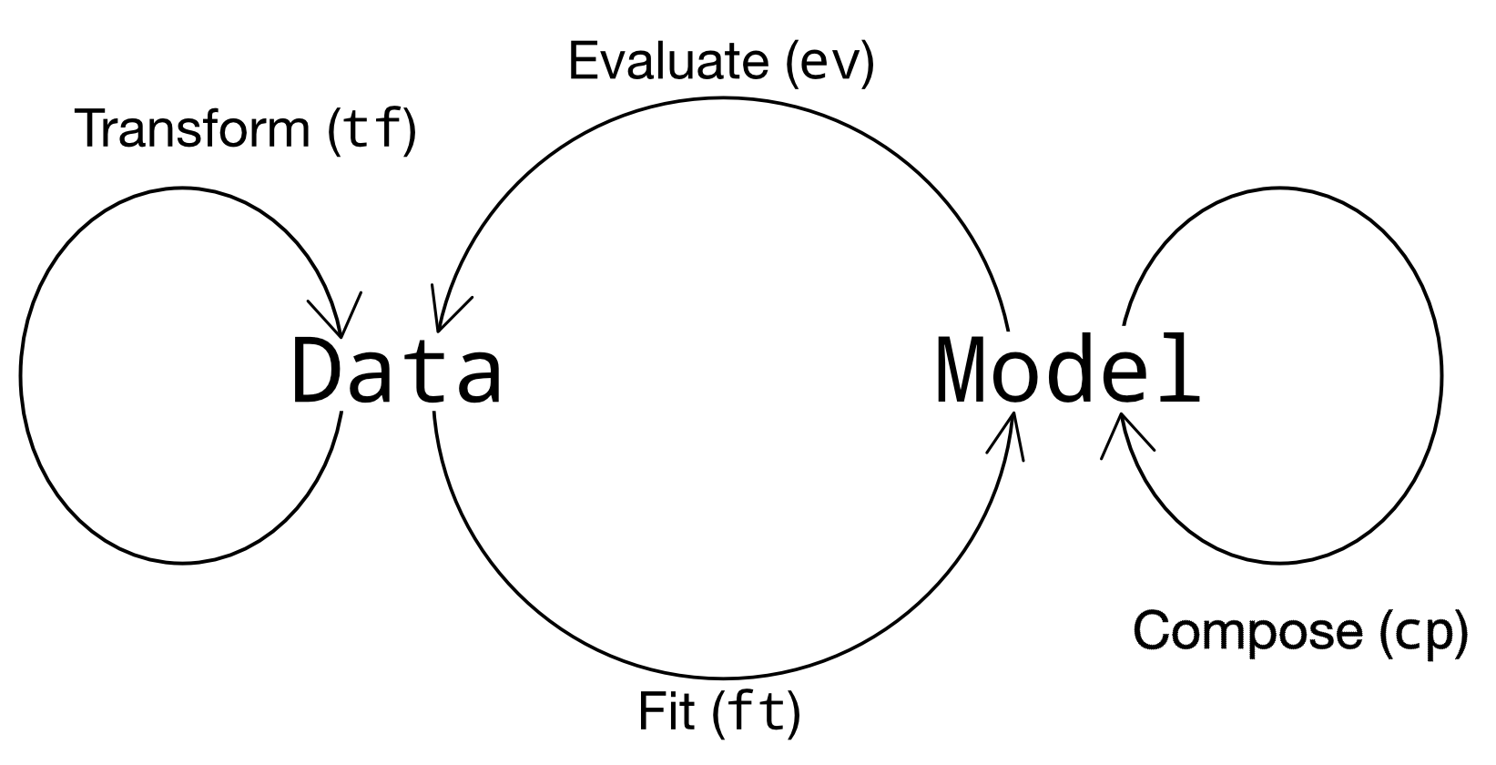
Recall that there are four classes of verb in grama; evaluation verbs take a model as an input and produce data as an output. Once we’ve generated that data, we can use visualization and other data tools to learn something about the model.

We’ll discuss three “subtypes” of evaluations:

• Manual input values - We specify the values for all of the inputs

• Mixed manual & automatic - We specify values for a subset of the inputs; the verb sets the remainder

• Automatic input values - The verb specifies all inputs values

Manual Input Values

There are two core evaluations—ev_df() and tf_md()—that require us to specify all the input values. These are manual but fundamental tools for working with a model.

DataFrame evaluation ev_df()

As the prefix implies, ev_df() takes a model as an input and returns data as an output. Since we need to specify all model input values, it is most convenient to pair ev_df() with the DataFrame constructor df_make(). Let’s talk about some practical considerations when putting these tools together.

q1 Set the input values

Use the gr.ev_df() verb with gr.df_make() to set input values for all the inputs of md_plate.

Hint: Note that there are a lot of variable values to set! Remember that “executing” a model on its own prints the model summary; use this to your advantage to get a reminder for what inputs you need, and what values might be reasonable.

# TASK: Complete the following code
(
    md_plate
    >> gr.ev_df(
        df=gr.df_make(
            m=1,
            t=0.06,
            h=12,
            w=12,
            L=1e-3,
            E=1e4,
            mu=0.33,
        )
    )
)

	m	t	h	w	L	E	mu	k_cr	g_buckle
0	1	0.06	12	12	0.001	10000.0	0.33	4.0	0.921591

Evaluation as transformation tf_md()

Evaluations enter into a pipeline in a specific way: an evaluation takes a model and returns a DataFrame. In some cases, it is useful to be able to “add” the results of a model to a DataFrame as a transform. The gr.tf_md() helper serves this functionality.

Let’s look at an example using the following dataset:

from grama.data import df_stang
df_stang.head(6)

	thick	alloy	E	mu	ang
0	0.022	al_24st	10600	0.321	0
1	0.022	al_24st	10600	0.323	0
2	0.032	al_24st	10400	0.329	0
3	0.032	al_24st	10300	0.319	0
4	0.064	al_24st	10500	0.323	0
5	0.064	al_24st	10700	0.328	0

q2 Use a model as a transform

Use gr.tf_md() to add model results to the following dataframe using md_plate.

(
    df_stang
    >> gr.tf_mutate(
        m=1,
        L=0.001,
        t=0.06,
        h=12,
        w=12,
    )
    >> gr.tf_md(md_plate)
)

	thick	alloy	E	mu	ang	m	L	t	h	w	k_cr	g_buckle
0	0.022	al_24st	10600	0.321	0	1	0.001	0.06	12	12	4.0	0.970579
1	0.022	al_24st	10600	0.323	0	1	0.001	0.06	12	12	4.0	0.971976
2	0.032	al_24st	10400	0.329	0	1	0.001	0.06	12	12	4.0	0.957800
3	0.032	al_24st	10300	0.319	0	1	0.001	0.06	12	12	4.0	0.941724
4	0.064	al_24st	10500	0.323	0	1	0.001	0.06	12	12	4.0	0.962794
...	...	...	...	...	...	...	...	...	...	...	...	...
71	0.064	al_24st	10400	0.327	90	1	0.001	0.06	12	12	4.0	0.956391
72	0.064	al_24st	10500	0.320	90	1	0.001	0.06	12	12	4.0	0.960722
73	0.081	al_24st	9900	0.314	90	1	0.001	0.06	12	12	4.0	0.901916
74	0.081	al_24st	10000	0.316	90	1	0.001	0.06	12	12	4.0	0.912317
75	0.081	al_24st	9900	0.314	90	1	0.001	0.06	12	12	4.0	0.901916

76 rows × 12 columns

Full-manual evaluation is important, but other grama verbs provide useful ways to automatically select input values.

Mixed Manual & Automatic

These verbs require that we set values for some of a model’s inputs. This is most commonly split across the deterministic and random variables: We set specific values for the deterministic inputs, and the verb handles the random inputs.

Nominal Evaluation

Sometimes it is useful to just get one set of “typical” values from a model. The gr.ev_nominal() verb provides this functionality.

q3 Evaluate at nominal values

Use gr.ev_nominal() to evaluate md_plate at nominal input values.

Hint: Consult the documentation to see how you can make a “default” choice for the deterministic inputs.

(
    md_plate
    >> gr.ev_nominal(df_det="nom")
)

	E	mu	w	m	t	L	h	k_cr	g_buckle
0	10344.736842	0.321363	12.0	3.0	0.075	0.0016	12.0	11.111111	4.116312

Sweeps

A key way to understand a model’s behavior is to sweep through values of the inputs and study the effects on the outputs. We can do this manually by specifying a grid of points with gr.df_grid(), or automatically with gr.ev_sinews().

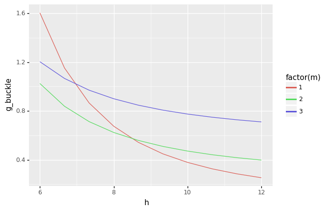
q4 Manual sweeps

Construct a manual sweep over values of m and h. Provide the values m = [1, 2, 3], and sweep h between 6 and 12.

Hint 1: Remember that in the previous exercise we learned how to use gr.df_grid() and gr.linspace(). To construct grids of points.

(
    md_plate
    >> gr.ev_nominal(
        df_det=gr.df_grid(
            w=12,
            t=1/32,
            L=0.0016,
            m=[1, 2, 3],
            h=gr.linspace(6, 12, 10)
        )
    )
    
    >> gr.ggplot(gr.aes("h", "g_buckle"))
    + gr.geom_line(gr.aes(color="factor(m)"))
)

<ggplot: (8766400696561)>

Note that you need to write a fair bit of code to produce a manual sweep. However, you also get complete control over which variables to sweep, and what ranges to consider.

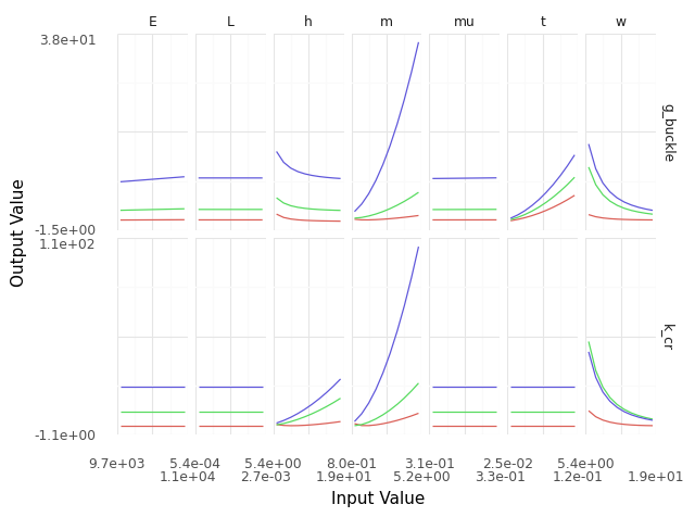
q5 Automatic sweeps

Use gr.ev_sinews() with df_det="swp" to sweep all the inputs in the model. Visualize the results.

(
    md_plate
    >> gr.ev_sinews(df_det="swp")
    >> gr.pt_auto()
)

Calling plot_sinew_outputs....

<ggplot: (8766400022477)>

Note how little code you need to write with gr.ev_sinews(); this is an excellent way to quickly inspect a model’s behavior. However, we don’t get as much control with this verb as with a manual sweep.

Automatic sweeps are useful for exploring a model, while manual sweeps are useful for getting more specific and especially for creating presentation-quality visuals to communicate results to others.

Random Sampling

Deterministic and random inputs are fundamentally different; deterministic inputs must be specified, while random inputs are fundamentally unknown in value. The verb gr.ev_sample() draws a random sample according to the random inputs, while handling the deterministic inputs according to the user’s choice.

q6 Evaluate a simple random sample

Use gr.ev_sample() to draw a sample of size 100. Use the nominal values for the deterministic inputs.

(
    md_plate
    >> gr.ev_sample(n=1e2, df_det="nom")
)

eval_sample() is rounding n...

	E	mu	w	m	t	L	h	k_cr	g_buckle
0	10445.410644	0.322644	12.0	3.0	0.075	0.0016	12.0	11.111111	4.160216
1	10535.972880	0.327419	12.0	3.0	0.075	0.0016	12.0	11.111111	4.210899
2	9963.545147	0.318756	12.0	3.0	0.075	0.0016	12.0	11.111111	3.957197
3	10444.887996	0.321367	12.0	3.0	0.075	0.0016	12.0	11.111111	4.156191
4	10645.085050	0.319009	12.0	3.0	0.075	0.0016	12.0	11.111111	4.228763
...	...	...	...	...	...	...	...	...	...
95	10219.180965	0.315176	12.0	3.0	0.075	0.0016	12.0	11.111111	4.048541
96	10564.800804	0.330628	12.0	3.0	0.075	0.0016	12.0	11.111111	4.232439
97	10400.542929	0.322074	12.0	3.0	0.075	0.0016	12.0	11.111111	4.140640
98	10960.709770	0.320350	12.0	3.0	0.075	0.0016	12.0	11.111111	4.358362
99	10335.834934	0.312982	12.0	3.0	0.075	0.0016	12.0	11.111111	4.088519

100 rows × 9 columns

Like gr.ev_sinews(), the verb gr.ev_nominal() works with gr.pt_auto() to produce quick visuals of model behavior. Combined with the skip keyword, this allows us to study both the input and output behavior of the model.

q7 Skip evaluation

Run the code below and inspect the output. Then add the keyword argument skip=True and re-run the code. Note the differences between the results. Answer the questions under observations below.

(
    md_plate
    >> gr.ev_sample(
        n=1e2, 
        df_det="nom",
        skip=True,
    )
    
    # NOTE: No need to edit
    >> gr.pt_auto()
)

eval_sample() is rounding n...
Design runtime estimates unavailable; model has no timing data.
Calling plot_scattermat....

Warning: Matplotlib is currently using module://matplotlib_inline.backend_inline, which is a non-GUI backend, so cannot show the figure.

Observations

• What values does g_buckle tend to take?

  • g_buckle tends to take values between 3.8 and 4.4

• How are the values for inputs E and mu related?

  • E and mu are positively correlated

Sweep Plus Sampling

Using gr.ev_sample() we can perform sweeps over deterministic inputs while sampling the random inputs. This follows similar code patterns to what we did with gr.ev_nominal().

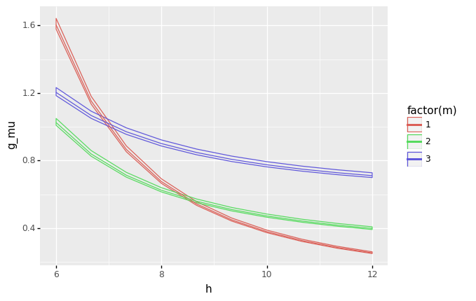
q8 Sweeps with sampling

Edit the code below to sweep over deterministic inputs, but sample the random inputs. Answer the questions under observations below.

(
    md_plate

    >> gr.ev_sample(
        n=1e2,
        df_det=gr.df_grid(
            w=12,
            t=1/32,
            L=0.0016,
            m=[1, 2, 3],
            h=gr.linspace(6, 12, 10)
        )
    )
    
    ## NOTE: No need to edit below; use to inspect results
    # Compute low, middle, high values at each m, h
    >> gr.tf_group_by(DF.m, DF.h)
    >> gr.tf_summarize(
        g_lo=gr.quant(DF.g_buckle, p=0.25),
        g_mu=gr.median(DF.g_buckle),
        g_hi=gr.quant(DF.g_buckle, p=0.75),
    )
    # Visualize
    >> gr.ggplot(gr.aes("h", "g_mu", color="factor(m)"))
    + gr.geom_ribbon(gr.aes(ymin="g_lo", ymax="g_hi"), fill=None)
    + gr.geom_line()
)

eval_sample() is rounding n...

<ggplot: (8766369982212)>

Observations

• How does the variability due to the random inputs (shown by width of bands) compare with variability due to the deterministic inputs (the curves).

  • The variability due to random inputs is much smaller than the variability due to deterministic inputs, but it is nonzero.

Automatic Input Values

Other grama verbs do not require us to specify any input values. Here are a few examples.

Contour Evaluation

In cases where we have just two inputs, we can construct contour plots of the output quantities. The verb gr.ev_contour() generates the data necessary for a contour plot.

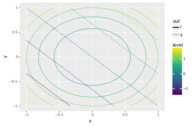
q9 Visualize function contours

Complete the arguments for gr.ev_contour() to generate contour data for the following model. Make sure to generate contours for both outputs f and g.

# TASK: Complete the contour evaluation arguments
(
    # NOTE: No need to edit this model
    gr.Model("Contour Demo")
    >> gr.cp_vec_function(
        fun=lambda df: gr.df_make(
            f=df.x**2 + df.y**2,
            g=df.x + df.y,
        ),
        var=["x", "y"],
        out=["f", "g"],
    )
    >> gr.cp_bounds(
        x=(-1, +1),
        y=(-1, +1),
    )
    
    # TASK: Complete the arguments for ev_contour()
    >> gr.ev_contour(

        var=["x", "y"],
        out=["f", "g"],
    )
    
    # NOTE: No need to edit; use to visualize
    >> gr.pt_auto()
)

Calling plot_contour....

<ggplot: (8766369610897)>

Note: Contours are fundamentally two-input constructions. If your model has more than two inputs, you will need to specify manual values for the other inputs.

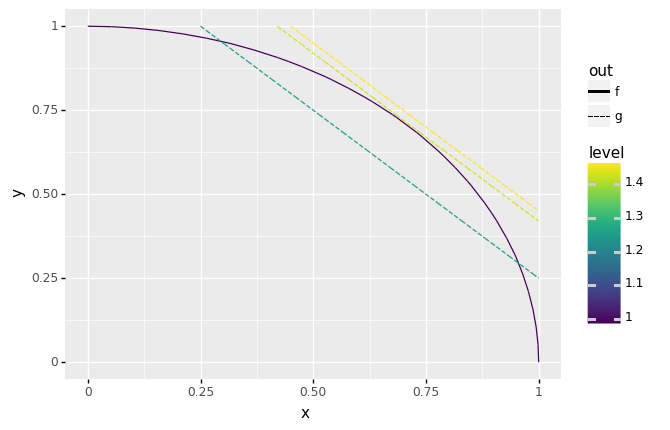
q10 Find specific contour levels

Use gr.ev_contour() to find the contour of g that is tangent to the contour where f == 1.

You’ll need to use the levels argument of gr.ev_contour() to do this, and it will take a bit of trial-and-error.

# TASK: Find the tangent contour of `g`
df_contour = (
    # NOTE: No need to edit this model
    gr.Model("Contour Demo")
    >> gr.cp_vec_function(
        fun=lambda df: gr.df_make(
            f=df.x**2 + df.y**2,
            g=df.x + df.y,
        ),
        var=["x", "y"],
        out=["f", "g"],
    )
    >> gr.cp_bounds(
        x=(0, +1),
        y=(0, +1),
    )
    
    # TASK: Use specific levels to find the tangent
    >> gr.ev_contour(
        var=["x", "y"],
        out=["f", "g"],

        levels=dict(
            f=[1],
            g=[1.25, 1.42, 1.45], # g == 1.42 is approximately correct
        )
    )
)

# NOTE: No need to edit; use to visualize
gr.plot_auto(df_contour)

Calling plot_contour....

<ggplot: (8766400432162)>

Constrained Minimization

As one last example of verbs that select automatic input values: Grama provides tools for constrained minimization, which determines the input values necessary to minimize an output quantity. The following code demonstrates how this works:

# NOTE: No need to edit
df_opt = (
    # Set up a model
    gr.Model("Contour Demo")
    >> gr.cp_vec_function(
        fun=lambda df: gr.df_make(
            f=df.x**2 + df.y**2,
            g=df.x + df.y - 1.42,
        ),
        var=["x", "y"],
        out=["f", "g"],
    )
    >> gr.cp_bounds(
        x=(0, +1),
        y=(0, +1),
    )
    
    # Minimize the objective with a constraint
    >> gr.ev_min(
        out_min="f",   # Output to minimize
        out_geq=["g"], # Output constraint, g >= 0
    )
)

df_opt

	y	x	y_0	x_0	f	g	success	message	n_iter
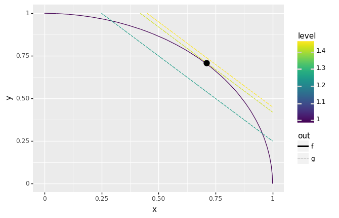
0	0.71	0.71	0.5	0.5	1.0082	1.776357e-15	True	Optimization terminated successfully	3

As a brief aside, this minimization is related to the “tangent” problem above.

# NOTE: No need to edit; this visualizes the optimization results
# in the context of the contour data
(
    df_contour
    >> gr.ggplot(gr.aes("x", "y"))
    + gr.geom_segment(
        gr.aes(
            xend="x_end", 
            yend="y_end",
            color="level",
            linetype="out",
          )
    )
    + gr.geom_point(data=df_opt, size=4)
)

<ggplot: (8766370353896)>

List of evaluation routines

For your reference, here are a few of the evaluation verbs, sorted by how they handle input values and with a brief description.

Verb	Input values	Description
ev_df()	Manual	DataFrame evaluation
tf_md()	Manual	Model as transformation
ev_nominal()	Mixed	Nominal values for random inputs
ev_sample()	Mixed	Random values for random inputs
ev_conservative()	Mixed	Conservative values for random inputs
ev_contour()	Auto	Generate contour plot data
ev_sinews()	Auto	Generate sinew plot data
ev_min()	Auto	Constrained minimization