Data: Deriving Quantities#

Purpose: Often our data will not tell us directly what we want to know; in these cases we need to derive new quantities from our data. In this exercise, we’ll work with tf_mutate() to create new columns by operating on existing variables, and use tf_group_by() with tf_summarize() to compute aggregate statistics (summaries!) of our data.

Aside: The data-summary verbs in grama are heavily inspired by the dplyr package in the R programming langauge.

Setup#

import grama as gr
DF = gr.Intention()
%matplotlib inline

# For assertion
from pandas.api.types import is_numeric_dtype

We’ll be using the diamonds as seen in e-vis00-basics earlier.

from grama.data import df_diamonds

Mutating DataFrames#

A mutation transformation allows us to make new columns (or edit old ones) by combining column values.

For example, let’s remember the diamonds dataset:

## NOTE: No need to edit
(
    df_diamonds
    >> gr.tf_head(5)
)

	carat	cut	color	clarity	depth	table	price	x	y	z
0	0.23	Ideal	E	SI2	61.5	55.0	326	3.95	3.98	2.43
1	0.21	Premium	E	SI1	59.8	61.0	326	3.89	3.84	2.31
2	0.23	Good	E	VS1	56.9	65.0	327	4.05	4.07	2.31
3	0.29	Premium	I	VS2	62.4	58.0	334	4.20	4.23	2.63
4	0.31	Good	J	SI2	63.3	58.0	335	4.34	4.35	2.75

If we wanted to approximate the volume of every diamond, we could do this by multiplying their x, y, and z dimensions. We could create a new column with this value via gr.tf_mutate():

## NOTE: No need to edit
(
    df_diamonds
    >> gr.tf_mutate(volume=DF.x * DF.y * DF.z)
    >> gr.tf_head(5)
)

	carat	cut	color	clarity	depth	table	price	x	y	z	volume
0	0.23	Ideal	E	SI2	61.5	55.0	326	3.95	3.98	2.43	38.202030
1	0.21	Premium	E	SI1	59.8	61.0	326	3.89	3.84	2.31	34.505856
2	0.23	Good	E	VS1	56.9	65.0	327	4.05	4.07	2.31	38.076885
3	0.29	Premium	I	VS2	62.4	58.0	334	4.20	4.23	2.63	46.724580
4	0.31	Good	J	SI2	63.3	58.0	335	4.34	4.35	2.75	51.917250

Aside: Note that we can use dot . notation to access columns, rather than bracket [] notation. This works only when the column names are valid variable names (i.e. do not contain spaces, do not contain special characters, etc.).

q1 Compute a mass density#

Approximate the density of the diamonds using the expression

\[\rho = \frac{\text{carat}}{xyz}.\]

Name the new column rho. Answer the questions under observations below.

## TASK: Provide the approximate density as the column `rho`
df_rho = (
    df_diamonds
    >> gr.tf_mutate(rho=DF["carat"] / DF["x"] / DF["y"] / DF["z"])
)

## NOTE: Use this to check your work
assert \
    "rho" in df_rho.columns, \
    "df_rho does not have a `rho` column"

assert \
    abs(df_rho.rho.median() - 6.117055e-03) < 1e-6, \
    "The values of df_rho.rho are incorrect; check your calculation"

print(
    df_rho
    >> gr.tf_filter(DF.rho < 1e6)
    >> gr.tf_select("rho")
    >> gr.tf_describe()
)

                rho
count  53920.000000
mean       0.006127
std        0.000178
min        0.000521
25%        0.006048
50%        0.006117
75%        0.006190
max        0.022647

Observations

What is the mean density rho?
- 0.006127
What is the lower-quarter density rho (25% value)?
- 0.006048
What is the upper-quarter density rho (75% value)?
- 0.006190

Vectorized Functions#

The gr.tf_mutate() verb carries out vector operations; these operations take in one or more columns, and return an entire column. For operations such as addition, this results in elementwise addition, as illustrated below:

`x`	`y`	`x + y`
1	0	1
1	1	2
1	-1	0

The gr.tf_mutate() verb accepts a wide variety of vectorized functions; the following table organizes these into various types of operations.

Type	Functions
Arithmetic ops.	`DF.x + 1, DF.y - DF.x, DF.x * DF.y, DF.x / DF.y, DF.x^DF.a`
Modular arith.	`DF.x // DF.y` (Floor division) `DF.x % DF.y` (Remainder)
Logical comp.	`<, <=, >, >=, !=, ==`
Logarithms	`gr.log(DF.x)`
Offsets	`gr.lead(DF.x), gr.lag(DF.x)`
Cumulants	`gr.cumsum(DF.x), gr.cumprod(DF.x), gr.cummin(DF.x), gr.cummaDF.x(DF.x), gr.cummean(DF.x)`
Ranking	`gr.min_rank(DF.x), gr.row_number(DF.x), gr.dense_rank(DF.x), gr.percent_rank(DF.x)`
Data conversion	`gr.as_numeric(DF.x)`, `gr.as_str(DF.x)`, `gr.as_factor(DF.x)`
Control	`gr.if_else()`, `gr.case_when()`

q2 Do a type conversion#

Convert the column y below into a numeric type.

Hint: Use the table above to find an appropriate data conversion function.

## TASK: Convert the `y` column to a numeric type
df_converted = (
    gr.df_make(
        x=[ 1, 2, 3],
        y=["4", "5", "6"],
    )

    >> gr.tf_mutate(y=gr.as_numeric(DF.y))
)

## NOTE: Use this to check your work
assert \
    is_numeric_dtype(df_converted.y), \
    "df_converted.y is not numeric; make sure to do a conversion"

print("Success!")

Success!

q3 Sanity-check the data#

The depth variable in df_diamonds is supposedly computed via depth_computed = 100 * 2 * DF["z"] / (DF["x"] + DF["y"]). Compute diff = DF["depth"] - DF["depth_computed"]: This is a measure of discrepancy between the given and computed depth. Answer the questions under observations below.

Hint: If you want to compute depth_computed and use it to compute diff, you’ll need to use two calls of gr.tf_mutate().

## TASK: Compute `depth_computed` and `diff`, as described above
df_depth = (
    df_diamonds 

# solution-begin    
    >> gr.tf_mutate(depth_computed=100 * 2 * DF["z"] / (DF["x"] + DF["y"]))
    >> gr.tf_mutate(diff = DF["depth"]- DF["depth_computed"])
)

## NOTE: Use this to check your work
assert \
    abs(df_depth["diff"].median()) < 1e-14, \
    "df_depth.diff has the wrong values; check your calculation"
assert \
    abs(df_depth["diff"].mean() - 5.284249e-03) < 1e-6, \
    "df_depth.diff has the wrong values; check your calculation"

# Show the data
(
    df_depth
    >> gr.tf_select("diff")
    >> gr.tf_describe()
)

	diff
count	5.393300e+04
mean	5.284249e-03
std	2.629223e+00
min	-5.574795e+02
25%	-2.660550e-02
50%	-7.105427e-15
75%	2.665245e-02
max	6.400000e+01

Observation

What is the mean of diff? What is the median of diff?
- mean(diff) == 5.284249e-03; median(diff) ~= 0.0
What are the min and max of diff?
- min(diff) == -5.574795e+02, max(diff) == 64
Remember that diff measures the agreement between depth and depth_computed; how well do these two quantities match?
- Generally, the agreement between depth and depth_computed is very good (the mean is close to zero, the 25% and 75% quantiles are quite small). However, there are some extreme cases of disagreement; perhaps there are data errors in these particular values?

Control Functions#

The gr.if_else() and gr.case_when() functions are special vectorized functions—they allow us to use more programming-like constructs to control the output. The gr.if_else() helper is a simple “yes-no” function, while gr.case_when() is a vectorized switch statement. If you are trying to do more complicated data operations, you might want to give these functions a look.

q4 Use an if/else statement#

Use gr.if_else() to flag diamonds as "Big" if they have carat >= 1 and "Small" otherwise.

Hint: Remember to read the documentation for an unfamiliar function to learn how to call it; in particular, try looking at the Examples section of the documentation.

## TODO: Compute the `size` using `gr.if_else()`
df_size = (
    df_diamonds
    >> gr.tf_mutate(
        
        size=gr.if_else(DF.carat >= 1, "Big", "Small")
    )
)

## NOTE: Use this to check you work
assert \
    "size" in df_size.columns, \
    "df_size does not have a `size` column"

assert \
    all(df_size[df_size["size"] == "Big"].carat >= 1), \
    "Size calculation is incorrect"

df_size

	carat	cut	color	clarity	depth	table	price	x	y	z	size
0	0.23	Ideal	E	SI2	61.5	55.0	326	3.95	3.98	2.43	Small
1	0.21	Premium	E	SI1	59.8	61.0	326	3.89	3.84	2.31	Small
2	0.23	Good	E	VS1	56.9	65.0	327	4.05	4.07	2.31	Small
3	0.29	Premium	I	VS2	62.4	58.0	334	4.20	4.23	2.63	Small
4	0.31	Good	J	SI2	63.3	58.0	335	4.34	4.35	2.75	Small
...	...	...	...	...	...	...	...	...	...	...	...
53935	0.72	Ideal	D	SI1	60.8	57.0	2757	5.75	5.76	3.50	Small
53936	0.72	Good	D	SI1	63.1	55.0	2757	5.69	5.75	3.61	Small
53937	0.70	Very Good	D	SI1	62.8	60.0	2757	5.66	5.68	3.56	Small
53938	0.86	Premium	H	SI2	61.0	58.0	2757	6.15	6.12	3.74	Small
53939	0.75	Ideal	D	SI2	62.2	55.0	2757	5.83	5.87	3.64	Small

53940 rows × 11 columns

Summarizing Data Frames#

The gr.tf_summarize() verb is used to reduce a DataFrame down to fewer rows using summary functions. For instance, we can compute the mean carat and price across the whole dataset of diamonds:

## NOTE: No need to edit
(
    df_diamonds
    >> gr.tf_summarize(
        carat_mean=gr.mean(DF.carat),
        price_mean=gr.mean(DF.price),
    )
)

	carat_mean	price_mean
0	0.79794	3932.799722

Notice that we went from having around 54,000 rows down to just one row; in this sense we have summarized the dataset.

Summary functions#

Summarize accepts a large number of summary functions; the table below lists and categorizes some of the most common summary functions.

Type	Functions
Location	`gr.mean(DF.x), gr.median(DF.x), gr.min(DF.x), gr.max(DF.x)`
Spread	`gr.sd(DF.x), gr.var(DF.x), gr.IQR(DF.x)`
Order	`gr.first(DF.x), gr.nth(DF.x, n), gr.last(DF.x)`
Counts	`gr.n_distinct(DF.x)`, `gr.n()` (Total count)
Logical	`gr.sum(DF.x == 0)` (Count cases where `x == 0`) `gr.pr(DF.g > 0)` (Probability helper)

q5 Count the Ideal rows#

Use gr.tf_summarize() to count the number of rows where cut == "Ideal". Provide this as the column n_ideal.

Hint: The Summary functions table above provides a recipe for counting the number of cases where some condition is met.

# TASK: Find the number of rows with cut == "Ideal"
df_nideal = (
    df_diamonds
    >> gr.tf_summarize(

        n_ideal=gr.sum(DF.cut == "Ideal")
    )
)

## NOTE: Use this to check your work
assert \
    "n_ideal" in df_nideal.columns, \
    "df_nideal does not have a `n_ideal` column"

assert \
    df_nideal["n_ideal"][0]/23==937,\
    "The count is incorrect"

df_nideal

	n_ideal
0	21551

Grouping by variables#

The gr.tf_summarize() verb is helpful for getting “basic facts” about a dataset, but it is even more powerful when combined with gr.tf_group_by().

The gr.tf_group_by() verb takes a DataFrame and “groups” it by one (or more) columns. This causes other verbs (such as gr.tf_summarize()) to treat the data as though it were multiple DataFrames; these sub-DataFrames exactly correspond to the groups determined by gr.tf_group_by().

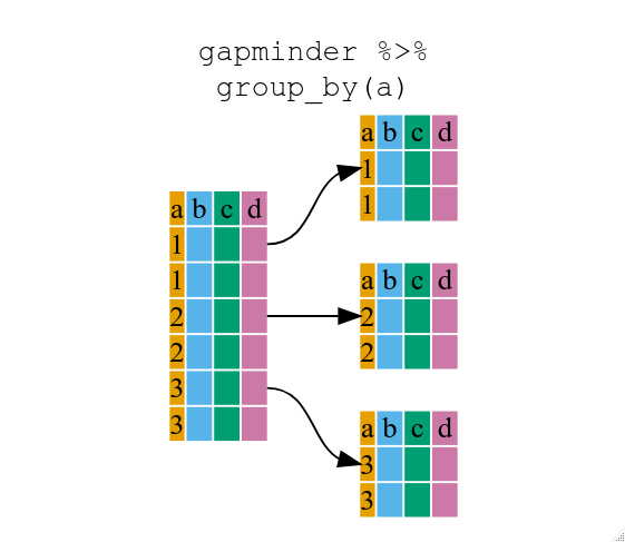
The verb modifies the behavior of a DataFrame to treat it as a collection of multiple datasets, defined by the grouping variable(s).

Image: Zimmerman et al.

When the input DataFrame is grouped, the gr.tf_summarize() verb will calculate the summary functions in a group-wise manner.

Grouped summarize

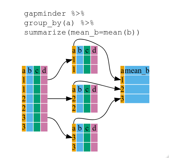
Image: Zimmerman et al.

Returning to the diamonds example: Let’s see what adding a gr.tf_group_by(DF.cut) before the price and carat mean calculation does to our results.

## NOTE: No need to edit
(
    df_diamonds
    >> gr.tf_group_by(DF.cut)
    >> gr.tf_summarize(
        carat_mean=gr.mean(DF.carat),
        price_mean=gr.mean(DF.price),
    )
)

	cut	carat_mean	price_mean
0	Fair	1.046137	4358.757764
1	Good	0.849185	3928.864452
2	Ideal	0.702837	3457.541970
3	Premium	0.891955	4584.257704
4	Very Good	0.806381	3981.759891

Now we can compare the mean carat and mean price across different cut levels. Personally, I was surprised to see that the Fair cut diamonds have a higher mean price than the Ideal diamonds!

q6 Try out a two-variable grouping#

The code below groups by two variables. Uncomment the tf_group_by() line below, and describe how the result changes.

#TASK: Uncomment the tf_group_by() below, and describe how the result changes
df_q2 = (
    df_diamonds

   >> gr.tf_group_by(DF["color"], DF["clarity"])
    >> gr.tf_summarize(diamonds_mean=gr.mean(DF["price"]))
)

df_q2

	clarity	color	diamonds_mean
0	I1	D	3863.023810
1	IF	D	8307.369863
2	SI1	D	2976.146423
3	SI2	D	3931.101460
4	VS1	D	3030.158865
5	VS2	D	2587.225692
6	VVS1	D	2947.912698
7	VVS2	D	3351.128391
8	I1	E	3488.421569
9	IF	E	3668.506329
10	SI1	E	3161.838005
11	SI2	E	4173.826036
12	VS1	E	2856.294301
13	VS2	E	2750.941700
14	VVS1	E	2219.820122
15	VVS2	E	2499.674067
16	I1	F	3342.181818
17	IF	F	2750.836364
18	SI1	F	3714.225716
19	SI2	F	4472.625233
20	VS1	F	3796.717742
21	VS2	F	3756.795093
22	VVS1	F	2804.276567
23	VVS2	F	3475.512821
24	I1	G	3545.693333
25	IF	G	2558.033774
26	SI1	G	3774.787449
27	SI2	G	5021.684109
28	VS1	G	4131.362197
29	VS2	G	4416.256498
30	VVS1	G	2866.820821
31	VVS2	G	3845.283437
32	I1	H	4453.413580
33	IF	H	2287.869565
34	SI1	H	5032.414945
35	SI2	H	6099.895074
36	VS1	H	3780.688623
37	VS2	H	4722.414486
38	VVS1	H	1845.658120
39	VVS2	H	2649.067434
40	I1	I	4302.184783
41	IF	I	1994.937063
42	SI1	I	5355.019663
43	SI2	I	7002.649123
44	VS1	I	4633.183992
45	VS2	I	5690.505560
46	VVS1	I	2034.861972
47	VVS2	I	2968.232877
48	I1	J	5254.060000
49	IF	J	3363.882353
50	SI1	J	5186.048000
51	SI2	J	6520.958246
52	VS1	J	4884.461255
53	VS2	J	5311.058824
54	VVS1	J	4034.175676
55	VVS2	J	5142.396947

Observations

How many rows does the commented version (no grouping) return?
- Just one row
How many rows (roughly) does the uncommented version (with grouping) return?
- Many rows! One row for every unique combination of clarity and color.

q7 Study the color#

Compute the mean price grouped by color. Answer the questions under observations below.

# TASK: Compute the mean price, grouped by color
(
    df_diamonds

# solution-begin    
    >> gr.tf_group_by(DF["color"])
    >> gr.tf_summarize(
        price_mean=gr.mean(DF["price"]),
    )
    
    ## NOTE: We need to "ungroup" in order to re-arrange the data
    >> gr.tf_ungroup()
    >> gr.tf_arrange("price_mean")
)

	color	price_mean
0	E	3076.752475
1	D	3169.954096
2	F	3724.886397
3	G	3999.135671
4	H	4486.669196
5	I	5091.874954
6	J	5323.818020

Observations

Which tends to be the most valuable color? Which is the least valuable?
- color == "J" tends to be the most valuable, while color == "E" tends to be least valuable.
The code above orders the colors according to their average price; are they in alphabetical order?
- Surprisingly, no! "D" would be the first letter, but color == "E" has the lowest mean price.

References#

Naupaka Zimmerman, Greg Wilson, Raniere Silva, Scott Ritchie, François Michonneau, Jeffrey Oliver, … Yuka Takemon. (2019, July). swcarpentry/r-novice-gapminder: Software Carpentry: R for Reproducible Scientific Analysis, June 2019 (Version v2019.06.1). Zenodo. http://doi.org/10.5281/zenodo.3265164

Data Science for Engineers

Data: Deriving Quantities

Contents

Data: Deriving Quantities#

Setup#

Mutating DataFrames#

q1 Compute a mass density#

Vectorized Functions#

q2 Do a type conversion#

q3 Sanity-check the data#

Control Functions#

q4 Use an if/else statement#

Summarizing Data Frames#

Summary functions#

q5 Count the Ideal rows#

Grouping by variables#

q6 Try out a two-variable grouping#

q7 Study the color#

References#