Demo Notebook 2022-06-27

Demos from the live sessions on 2022-06-27.

Setup

Ye olde setup chunk below.

import grama as gr
import pandas as pd
DF = gr.Intention()
%matplotlib inline

# For downloading data
import os
import requests

Download the michelson data.

# Filename for local data
filename_data = "../challenges_assignment/data/michelson.csv"

# The following code downloads the data, or (after downloaded)
# loads the data from a cached CSV on your machine
if not os.path.exists(filename_data):
    # Make request for data
    url_data = "https://docs.google.com/spreadsheets/d/1av_SXn4j0-4Rk0mQFik3LLr-uf0YdA06i3ugE6n-Zdo/export?format=csv"
    r = requests.get(url_data, allow_redirects=True)
    open(filename_data, 'wb').write(r.content)
    print("   Data downloaded from public Google sheet")
else:
    # Note data already exists
    print("   Data loaded locally")
    
# Read the data into memory
df_michelson = (
    pd.read_csv(filename_data)
    >> gr.tf_select("Date", "Distinctness", "Temp", "Velocity")
)

# Adjust values
df_q2 = (
    df_michelson
    >> gr.tf_mutate(VelocityVacuum=DF.Velocity + 92)
)

   Data loaded locally

## NOTE: Don't edit; these are constants used in the challenge
LIGHTSPEED_VACUUM    = 299792.458 # Exact speed of light in a vacuum (km / s)
LIGHTSPEED_MICHELSON = 299944.00  # Michelson's speed estimate (km / s)
LIGHTSPEED_PM        = 51         # Michelson error estimate (km / s)

Temperature dependence

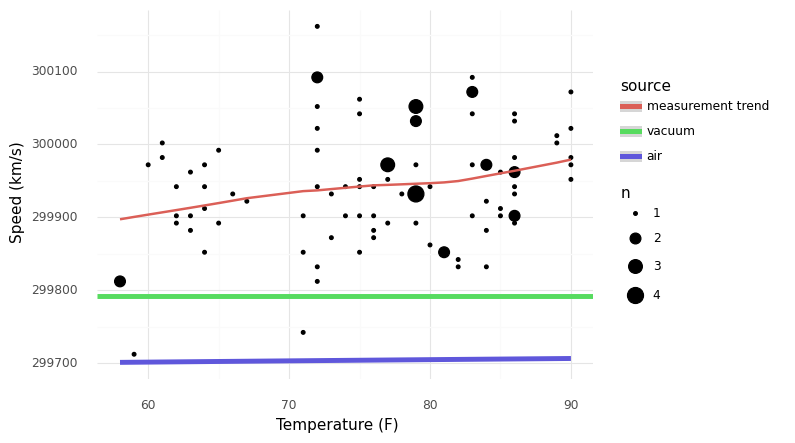
Part of what makes analyzing the Michelson data difficult—and not fooling ourselves into seeing spurious patterns—is that the speed of light (in air) does have a temperature dependence. Let’s compare that dependence to the observed trend in the data.

For temperature, I’m pulling an index-of-refraction calculation for air to adjust the speed-of-light from vacuum to that in air.

(
    df_q2
    >> gr.ggplot(gr.aes("Temp", "VelocityVacuum"))
    + gr.geom_count()
    + gr.geom_smooth(
        data=df_q2
        >> gr.tf_mutate(source="measurement trend"),
        mapping=gr.aes(color="source"),
    )
    + gr.geom_hline(
        data=gr.df_make(c_vacuum=[LIGHTSPEED_VACUUM], source="vacuum"),
        mapping=gr.aes(yintercept="c_vacuum", color="source"),
        size=2,
    )
    + gr.geom_line(
        data=df_q2
        >> gr.tf_mutate(T_K=(DF.Temp - 32) * 5/9 + 273.15) # Convert T to kelvin
        >> gr.tf_mutate(n=1 + 0.000293 * 300 / DF.T_K)     # Compute index of refraction
        >> gr.tf_mutate(c_air=LIGHTSPEED_VACUUM / DF.n)    # Compute speed in air
        >> gr.tf_mutate(source="air"),
        mapping=gr.aes(y="c_air", color="source"),
        size=2,
    )
    + gr.theme_minimal()
    + gr.labs(
        x="Temperature (F)",
        y="Speed (km/s)",
    )
)

/Users/zach/opt/anaconda3/envs/evc/lib/python3.9/site-packages/plotnine/stats/smoothers.py:310: PlotnineWarning: Confidence intervals are not yet implementedfor lowess smoothings.

<ggplot: (8790976147962)>

As we can see, the measurement trend in temperature is much steeper than the real trend in air. This suggests that much of the variation in temperature that we see is erroneous (not real).

One of the challenges in making this kind of determination is that what is real and what is erroneous depends on what we are trying to study. While temperature does affect the speed of light in air, it does not affect the speed of light in a vacuum. Let’s compare a couple of physical mechanisms, and note whether they are real or error for different quantities:

Physical mechanism	For lightspeed in air	For lightspeed in vacuum
Miscalibrated instrument	Error	Error
Temperature changes index of refraction of air	Real	Error