Demo Notebook 2022-07-18#

Demos from the live sessions on 2022-07-18.

Setup#

import grama as gr
import pandas as pd
import numpy as np
DF = gr.Intention()
%matplotlib inline

Load the challenge data#

df_data = pd.read_csv("../challenges/data/c05-data.csv")
df_data

	E	mu	t	id_machine	id_specimen	id_measurement
0	10113.457096	0.319442	0.250	A	0	g
1	9432.148720	0.308230	0.250	A	1	g
2	10468.172283	0.328422	0.250	A	2	g
3	9474.697920	0.333919	0.250	A	3	g
4	10010.402837	0.310751	0.250	A	4	g
...	...	...	...	...	...	...
715	11935.167126	0.319328	0.125	F	115	l
716	11552.946124	0.317546	0.125	F	116	l
717	11985.579932	0.332173	0.125	F	117	l
718	12092.949690	0.317655	0.125	F	118	l
719	12170.319166	0.335891	0.125	F	119	l

720 rows × 6 columns

Compare across thicknesses#

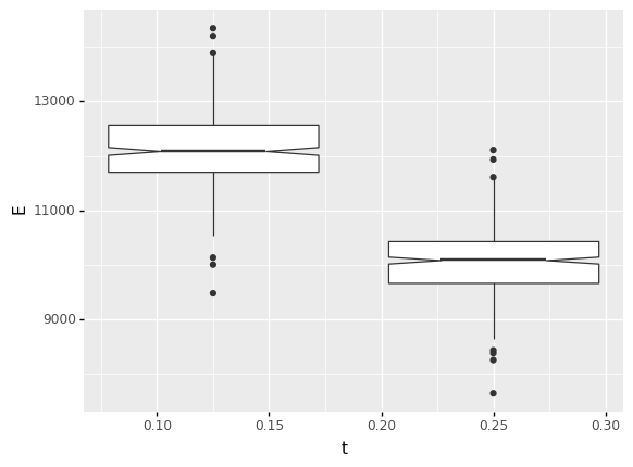
I chose to make this comparison using boxplots. These are a simple (and underrated!) way to make comparisons across groups.

A particularly helpful tip is to use notch=True with boxplots. This visualizes a confidence interval on the median (the middle line), which is helpful for assessing the statistical signifance of differences. As we can see from the boxplots below, the two notches are highly separated, suggesting that the difference is statistically significant (not likely to be due to chance alone).

## TODO: Compare elasticity across thicknesses
## NOTE: There are many ways to do this!
(
    df_data
# solution-begin
    >> gr.ggplot(gr.aes("t", "E"))
    + gr.geom_boxplot(gr.aes(group="t"), notch=True)
# solution-end
)

<ggplot: (8770214991553)>

Explore the experimental design#

(The following is the solution code from the q2 task.)

Answer the following questions to better understand the experimental design. Note that the same questions are posed within each cell and under observations below.

Hint: The verbs tf_count() and tf_distinct() will be very useful for answering some of these questions!

## Q: What thicknesses were tested?
# solution-begin
(
    df_data
    >> gr.tf_count(DF.t)
)
# solution-end

	t	n
0	0.125	360
1	0.250	360

## Q: How many unique specimens were manufactured?
# solution-begin
(
    df_data
    >> gr.tf_summarize(spec_max=gr.max(DF.id_specimen) + 1)
)
# solution-end

	spec_max
0	120

## Q: How many specimens were made on each machine?
# solution-begin
(
    df_data
    >> gr.tf_distinct(DF.id_specimen, DF.id_machine)
    >> gr.tf_count(DF.id_machine)
)
# solution-end

	id_machine	n
0	A	20
1	B	20
2	C	20
3	D	20
4	E	20
5	F	20

## Q: How many times did each operator measure each specimen?
# solution-begin
(
    df_data
    >> gr.tf_count(DF.id_specimen, DF.id_measurement)
    >> gr.tf_summarize(n_max=gr.max(DF.n))
)
# solution-end

	n_max
0	1

Observations

What thicknesses were tested?
- (Your response here)
How many unique specimens were manufactured?
- (Your response here)
How many specimens were made on each machine?
- (Your response here)
How many times did each operator measure each specimen?
- (Your response here)

What thicknesses were tested?
- 0.125 and 0.250 inches
How many unique specimens were manufactured?
- 120
How many specimens were made on each machine?
- 20 specimens each
How many times did each operator measure each specimen?
- Just once

Fitting a lognorm#

First, let’s set up the data as it was in the challenge. We seek to model the variability of E as observed in df_sub.

## NOTE: No need to edit
df_sub = (
    df_data
    >> gr.tf_filter(
        DF.t == 0.250,
        DF.id_machine != "C",
        DF.id_measurement != "h",
    )
)

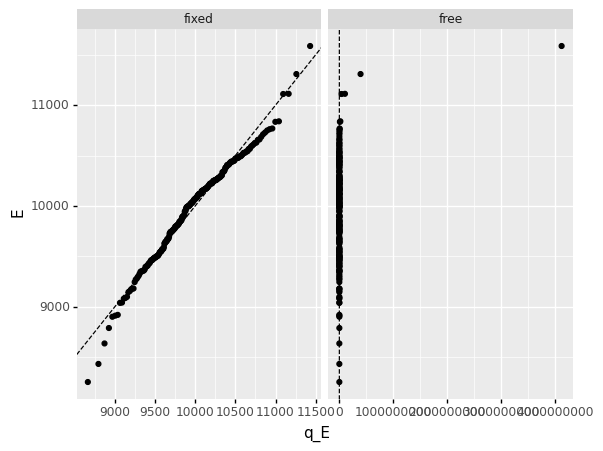
The following code fits a lognormal distribution to the observations on E.

Note that the "lognorm" distribution in grama uses the scipy implementation. As noted in that documentation, the loc and scale parameters are used to modify the input variable (x - loc) / scale. However, we can freeze the location parameter of the distribution by setting floc=0. This is useful when fitting a lognormal distribution becomes unstable. The following code demonstrates this phenomenon:

## Fit with loc == 0
mg_fixed = gr.marg_fit(
    "lognorm", 
    df_sub.E, 
    floc=0,
)

## Fit with loc able to move
mg_free = gr.marg_fit(
    "lognorm", 
    df_sub.E, 
    # floc=0, # Don't set the location parameter to zero
)

## Use QQ plot to asses
(
    df_sub
    >> gr.tf_mutate(
        fixed=gr.qqvals(DF.E, marg=mg_fixed),
        free=gr.qqvals(DF.E, marg=mg_free),
    )
    >> gr.tf_pivot_longer(
        columns=["fixed", "free"],
        names_to="location",
        values_to="q_E",
    )
    
    >> gr.ggplot(gr.aes("q_E", "E"))
    + gr.geom_abline(intercept=0, slope=1, linetype="dashed")
    + gr.geom_point()
    + gr.facet_grid("~location", scales="free_x")
)

/Users/zach/opt/anaconda3/envs/evc/lib/python3.9/site-packages/plotnine/facets/facet.py:487: FutureWarning: Passing a set as an indexer is deprecated and will raise in a future version. Use a list instead.
/Users/zach/opt/anaconda3/envs/evc/lib/python3.9/site-packages/plotnine/utils.py:371: FutureWarning: The frame.append method is deprecated and will be removed from pandas in a future version. Use pandas.concat instead.
/Users/zach/opt/anaconda3/envs/evc/lib/python3.9/site-packages/plotnine/utils.py:371: FutureWarning: The frame.append method is deprecated and will be removed from pandas in a future version. Use pandas.concat instead.

<ggplot: (8770231222013)>

Clearly the free option has resulted in a terrible fit!

We can also see that the fitted parameter values for the free version have ended up being enormous (and implausible).

print(mg_fixed)  # floc == 0 (fixed)
print(mg_free)   # floc free

(+0) lognorm, {'mean': '9.965e+03', 's.d.': '4.977e+02', 'COV': 0.05, 'skew.': 0.15, 'kurt.': 3.04}
(+0) lognorm, {'mean': '2.409e+13', 's.d.': '3.298e+26', 'COV': 13691416095072.72, 'skew.': 2.5665226910475562e+39, 'kurt.': 1.2347725193581465e+105}

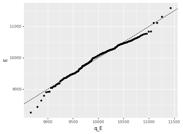
Real variability?#

Note that the tails of the fitted distribution seem to exhibit some mismatch:

(
    df_sub
    >> gr.tf_mutate(
        q_E=gr.qqvals(DF.E, marg=mg_fixed),
    )
    
    >> gr.ggplot(gr.aes("q_E", "E"))
    + gr.geom_abline(intercept=0, slope=1, linetype="dashed")
    + gr.geom_point()
)

<ggplot: (8770214991071)>

This is a problem for us, as we’re aiming to assess probabilities that lie in the tails (around the 1% level).

Part of the issue here is that the real and erroneous variability mingle to create a complicated, non-standard distribution. We can improve the situation by applying the mean heuristic to the data:

## NOTE: No need to edit
df_real = (
    df_sub
    >> gr.tf_group_by(DF.id_specimen)
    >> gr.tf_summarize(
        mu=gr.mean(DF.mu),
        E=gr.mean(DF.E),
    )
    >> gr.tf_ungroup()
)

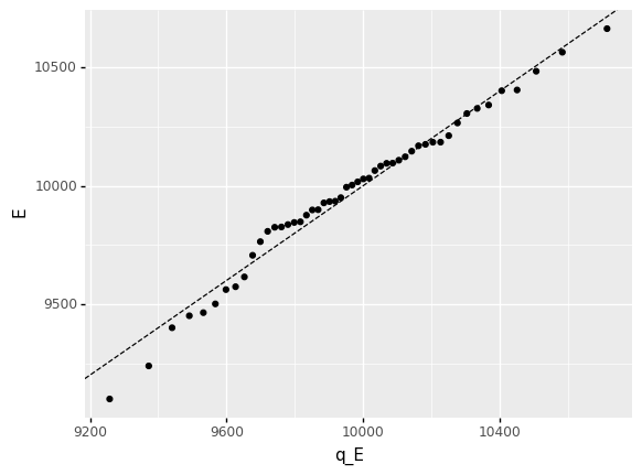
Now re-fit the marginal distribution on the reduced dataset:

# solution-begin
mg_E = gr.marg_fit(
    "lognorm", 
    df_real.E, 
    floc=0,
)

(
    df_real
    >> gr.tf_mutate(
        q_E=gr.qqvals(DF.E, marg=mg_E),
    )
    
    >> gr.ggplot(gr.aes("q_E", "E"))
    + gr.geom_abline(intercept=0, slope=1, linetype="dashed")
    + gr.geom_point()
)
# solution-end

<ggplot: (8770215282339)>

As discussed in the morning session, this fit is still not perfect. However, we can see that the points generally lie closer to the line than before.

Since the real variability actually was generated from a lognormal distribution, the remaining mismatch here is due to erroneous (sampling) variability. Dealing with this remaining uncertainty is outside the scope of this course, but you can take a look at the Further Reading below for more information!

Data Science for Engineers

Demo Notebook 2022-07-18

Contents