Grama: Fitting Univariate Distributions

Purpose: As we’ve seen through studying a lot of datasets, many physical systems exhibit variability and other forms of uncertainty. Thus, it is beneficial to be able to model uncertainty using distributions. In this two-part exercise, we’ll first learn how to fit a distribution for a single quantity, then learn how to deal with multiple related quantities.

In the final exercise e-grama08-duu we’ll see how to use a distribution model to do useful engineering work.

Setup

import grama as gr
DF = gr.Intention()
%matplotlib inline

For this exercise, we’ll study a dataset of observations on die cast aluminum parts.

## NOTE: No need to edit
from grama.data import df_shewhart

Why fit a distribution?

Before we start fitting distributions: Why would we ever want to fit a distribution?

As we’ve seen from studying a large number of datasets, most engineering data exhibit variability. If the variability is real, it can have real impacts on the engineering systems we design.

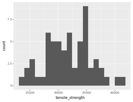
For instance, here’s a dataset of realized aluminum tensile strength values:

# NOTE: No need to edit; run and inspect
(
    df_shewhart
    >> gr.ggplot(gr.aes("tensile_strength"))
    + gr.geom_histogram(bins=20)
)

<ggplot: (8758216577434)>

Clearly, these data exhibit variability—they do not take a single value.

Dangers of assuming the mean

Why don’t we just take the mean of tensile_strength and use that for design? It turns out this approach is very dangerous when safety is a consideration. Let’s take a look at the tensile strength of an aluminum alloy.

# NOTE: No need to edit; run and inspect
(
    df_shewhart
    >> gr.ggplot(gr.aes("tensile_strength"))
    + gr.geom_histogram(bins=20)
    + gr.geom_vline(
        data=df_shewhart
        >> gr.tf_summarize(tensile_strength=gr.mean(DF.tensile_strength)),
        mapping=gr.aes(xintercept="tensile_strength"),
        linetype="dashed",
    )
)

<ggplot: (8758214365901)>

Clearly, values of tensile_strength tend to land both above and below the mean. But what ramifications does this have for engineering design?

q1 What fraction of tensile_strength is below the mean?

Compute the fraction of observations in df_shewhart where tensile_strength < mean(tensile_strength). Answer the questions under observations below.

## TASK: Compute the fraction of values where tensile_strength < mean(tensile_strength)
(
    df_shewhart
    >> gr.tf_summarize(
        frac=gr.pr(DF.tensile_strength < gr.mean(DF.tensile_strength))
    )
)

	frac
0	0.5

Observations

For these questions, assume the variability in tensile_strength is real; that is, the variability is not simply due to measurement error.

• What fraction of observations have tensile_strength < mean(tensile_strength)?

  • I find that frac == 0.5 (i.e. 50%)

• Suppose a design assumed mean(tensile_strength) as the design stress; that is, every part would be subject to a stress equal to mean(tensile_strength). The fraction you computed above would be the fraction of parts that would fail. Would this failure rate be acceptable for any engineering system involving human safety?

  • Absolutely not; a failure rate of 50% would be completely unacceptable for any application involving human safety.

Rather than just assume a fixed value for tensile_strength, we can model it as uncertain and design around that uncertainty. We’ll learn how to make engineering decisions under uncertainty in a future exercise; for now, let’s focus on the modeling steps.

Random variables

Clearly tensile_strength does not take a single value; therefore, we should think of tensile_strength as a random variable. A random variable is a mathematical object that we can use to model an uncertain quantity. Unlike a deterministic variable that has one fixed value (say \(x = 1\)), a random variable can take a different value each time we observe it. For instance, if \(X\) were a random variable, and we used \(X_i\) to denote the value that occurs on the \(i\)-th observation, then we might see a sequence like

\[X_1 = 1, X_2 = -3, X_3 = 1, X_4 = 5, \dots\]

What counts as an observation depends on what we are using the random variable to model. Essentially, an observation is an occurrence that gives us the potential to “see” a new value.

Let’s take a look at the tensile_strength example to get a better sense of these ideas.

For the tensile_strength, we saw a sequence of different values:

## NOTE: No need to edit
(
    df_shewhart
    >> gr.tf_head(4)
)

	specimen	tensile_strength	hardness	density
0	1	29314	53.0	2.666
1	2	34860	70.2	2.708
2	3	36818	84.3	2.865
3	4	30120	55.3	2.627

Every time we manufacture a new part, we perform a sequence of manufacturing steps that work together to “lock in” a particular value of tensile_strength. Those individual steps tend to go slightly differently each time we make a part (e.g. an operator calls in sick one day, we get a slightly more dense batch of raw material, it’s a particularly hot summer day, etc.), so we end up with different properties in each part.

Given the complicated realities of manfacturing, it makes sense to think of an observation as being one complete run of the manufacturing process that generates a particular part with its own tensile_strength. This is what the specimen column in df_shewhart refers to; a unique identifier tracking individual runs of the complete manufacturing process, resulting in a unique part.

Nomenclature: A realization is like a single roll of a die

Some nomenclature: When we talk about random quantities, we use the term realization (or observation) to refer to a single event that yields a random value, according to a particular distribution. For instance, a single manufactured part will have a realized strength value. If we take multiple realizations, we will tend to see different values. For instance, we saw a large amount of variability among the realized tensile_strength values above.

A single realization tells us very little about how the distribution tends to behave, but a set of realizations (a sample) will give us a sense of how the random values tend to behave collectively. A distribution is a way to model that collective behavior.

A distribution defines a random variable

As we saw in e-stat04-distributions, we can use distributions to quantitatively describe an uncertain quantity. A distribution defines a random variable. We say that a random variable \(X\) is distributed according to a particular density \(\rho\), and we express the same statement mathematically as

\[X \sim \rho.\]

We learned how to compute useful quantities using distributions in e-stat04-distributions; in the rest of this exercise, we’ll learn how to fit a distribution in order use information from a dataset to model observations from the physical world.

The steps to fitting

1. Check for statistical control

2. Select candidate distributions

3. Fit and assess

1. Check for statistical control

Sometimes the variability we see in a dataset can be explained; in this case, we shouldn’t just model it as random—we should work to understand why we saw that variability, and try to eliminate that source of variation. As we saw in e-stat06-spc, we can use control charts to hunt for explainable sources of variability.

If we find no explainable sources of variability in a dataset, we can provisionally declare that the data are under statistical control, and model the variability as random.

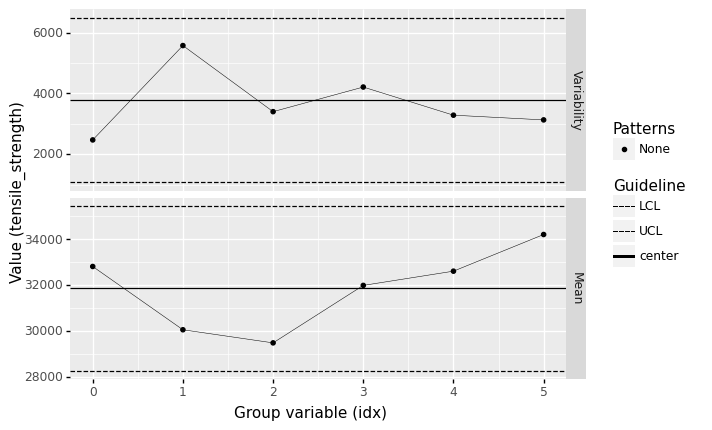
q2 Assess statistical control

Assess the state of statistical control of tensile_strength using an X-bar and S chart. Answer the questions under observations below.

Hint: You did this at the end of e-stat06-spc; see that exercise for a refresher if you need it.

## TASK: Assess statistical control with an Xbar and S chart
(
    df_shewhart
    >> gr.tf_mutate(idx=DF.index // 10)
    >> gr.pt_xbs(group="idx", var="tensile_strength")
)

/home/zach/Git/py_grama/grama/tran_pivot.py:570: SettingWithCopyWarning: 
A value is trying to be set on a copy of a slice from a DataFrame

See the caveats in the documentation: https://pandas.pydata.org/pandas-docs/stable/user_guide/indexing.html#returning-a-view-versus-a-copy
/home/zach/Bin/anaconda3/envs/evc/lib/python3.9/site-packages/plotnine/utils.py:371: FutureWarning: The frame.append method is deprecated and will be removed from pandas in a future version. Use pandas.concat instead.
/home/zach/Bin/anaconda3/envs/evc/lib/python3.9/site-packages/plotnine/utils.py:371: FutureWarning: The frame.append method is deprecated and will be removed from pandas in a future version. Use pandas.concat instead.
/home/zach/Bin/anaconda3/envs/evc/lib/python3.9/site-packages/plotnine/utils.py:371: FutureWarning: The frame.append method is deprecated and will be removed from pandas in a future version. Use pandas.concat instead.

<ggplot: (8758214107194)>

Observations

• What assumptions did you need to make to construct a control chart?

  • I had to assume that the observations were reported in their run-order. I also chose to group in batches of n_batch = 10 to help ensure the batch means follow the CLT.

• Does tensile_strength seem to be under statistical control?

  • According to a batch size of n_batch = 10, yes.

If the data seem to be under statistical control, then we can model the measured value as random. For this exercise, we’ll assume that tensile_strengh is under statistical control and proceed with modeling.

2. Select candidate distributions

Once we’ve decided to proceed modeling a quantity as random, we next need to select candidate distributions to represent the quantity. This is a process that should involve critical thinking about the physical quantity.

(Short) list of distributions

The following is a short list of distributions, along with a short description for each. The description information is helpful for choosing candidate distributions.

Distribution	Name	Description
Normal (Gaussian)	"norm"	symmetric; infinite extent
Lognormal	"lognorm"	asymmetric; semi-infinite (positive)
Uniform	"uniform"	flat, bounded
Beta	"beta"	flexible shape, bounded
Weibull	"weibull_min"	asymmetric; semi-infinite (positive)

For a longer list of supported distributions, see the scipy documentation for continuous distributions.

q3 Select reasonable distributions for tensile_strength

From the list above, select a few reasonable distributions that could describe the tensile_strength.

List the distributions below:

• Lognormal - strength is non-negative

• Weibull - strength is non-negative

3. Fit and assess

Now that we’ve selected reasonable distributions for our quantity, we can fit and assess the distributions.

Grama tools for fitting

Grama provides two ways to fit a distribution:

Verb	Purpose
gr.marg_mom()	Fit a distribution based on a handful of statistics, e.g. mean and variance
gr.marg_fit()	Fit a distribution using multiple observations, e.g. df_shewhart.tensile_strength

Let’s learn how to use both!

q4 Fit a normal distribution

Complete the arguments for both gr.marg_mom() and gr.marg_fit() below to fit a normal distribution for the tensile_strength.

Hint 1: Remember the table above (Short list of distributions) lists the string names for a set of distributions.

Hint 2: Remember to use the documentation to learn how to call a new function!

## TASK: Complete the arguments for the two functions below
mg_mom = gr.marg_mom(

    "norm", 
    mean=df_shewhart.tensile_strength.mean(),
    var=df_shewhart.tensile_strength.var(),
)

mg_fit = gr.marg_fit(

    "norm",
    df_shewhart.tensile_strength,
)

## NOTE: No need to edit; this will run when you complete the task
print(mg_mom)
print(mg_fit)

(+0) norm, {'mean': '3.187e+04', 's.d.': '3.996e+03', 'COV': 0.13, 'skew.': 0.0, 'kurt.': 3.0}
(+0) norm, {'mean': '3.187e+04', 's.d.': '3.963e+03', 'COV': 0.12, 'skew.': 0.0, 'kurt.': 3.0}

QQ plots

A QQ plot is a statistical tool for assessing the quality of a distribution fit. A QQ plot visualizes the quantiles of the dataset against the quantiles of the fitted distribution: A perfect fit will have all points fall along the line \(y = x\).

The grama helper gr.qqvals() is used within a call to gr.tf_mutate(); we use gr.qqvals() to compute the theoretical quantiles for a QQ plot.

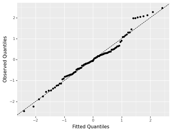
q5 Inspect a “perfect” QQ plot

The following code draws a sample from a normal distribution, then assesses a normal fit of that dataset using a QQ plot. Run the code, inspect the plot, then answer the questions under observations below.

## NOTE: No need to edit; run and inspect
# Define a standard normal distribution
mg_norm = gr.marg_mom("norm", mean=0, sd=1)

(
    # Draw some random values
    gr.df_make(z=mg_norm.r(100))
    # Compute theoretical quantiles based on fitted normal
    >> gr.tf_mutate(q=gr.qqvals(DF.z, "norm"))
    
    # Visualize
    >> gr.ggplot(gr.aes("q", "z"))
    # Add a guideline
    + gr.geom_abline(intercept=0, slope=1, linetype="dashed")
    
    + gr.geom_point()
    + gr.labs(x="Fitted Quantiles", y="Observed Quantiles")
)

<ggplot: (8758213920317)>

Observations

• How “straight” do the observations appear?

  • Quite straight, but not perfect! Note that the observations are a bit “jittered” in the middle, and and fall progressively far from the line \(y=x\) at the tails of the distribution. Keep in mind that this is what a perfectly chosen distribution will look like on a QQ plot; the plot above (with all of its imperfections) is what the best possible fit will look like!

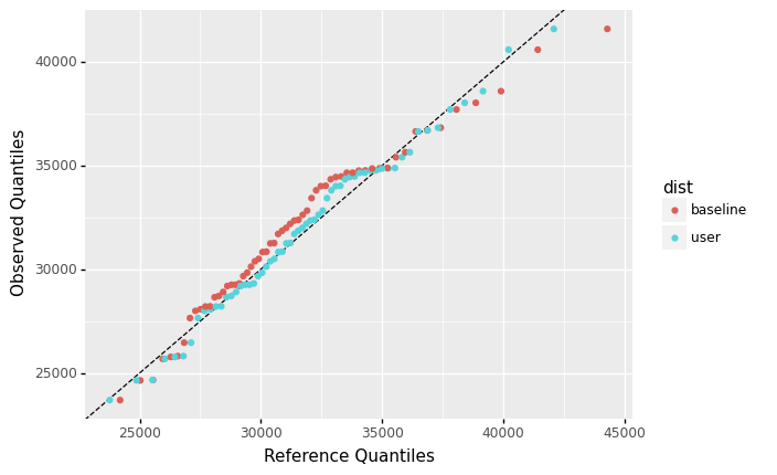
q6 Fit a distribution for the tensile_strength

Pick a distribution from the list of “reasonable” distributions you generated in __q3__ Select reasonable distributions, and fit a distribution for df_shewhart.tensile_strength. Answer the questions under observations below.

Hint: If you choose to fit a "lognorm" or "weibull_min", you may find it helpful to set the keyword argument floc=0 to use the 2-parameter version of the distribution. Anecdotally, I find the 2-parameter version to be more stable for small datasets.

# TASK: Fit a distribution for the tensile_strength;
# assign it to mg_user below

mg_user = gr.marg_fit(
    "lognorm", 
    df_shewhart.tensile_strength,
    floc=0,
)
# NOTE: Don't edit this; use to check your results
mg_base = gr.marg_fit(
    "gengamma",
    df_shewhart.tensile_strength,
    floc=0,
)

(
    df_shewhart
    >> gr.tf_mutate(
        q_baseline=gr.qqvals(DF.tensile_strength, marg=mg_base),
        q_user=gr.qqvals(DF.tensile_strength, marg=mg_user),
    )
    >> gr.tf_pivot_longer(
        columns=gr.contains("q_"),
        names_to=[".value", "dist"],
        names_sep="_",
    )
    
    >> gr.ggplot(gr.aes("q", "tensile_strength", color="dist"))
    + gr.geom_abline(intercept=0, slope=1, linetype="dashed")
    + gr.geom_point()
    + gr.labs(x="Reference Quantiles", y="Observed Quantiles")
)

/home/zach/Git/py_grama/grama/tran_pivot.py:570: SettingWithCopyWarning: 
A value is trying to be set on a copy of a slice from a DataFrame

See the caveats in the documentation: https://pandas.pydata.org/pandas-docs/stable/user_guide/indexing.html#returning-a-view-versus-a-copy

<ggplot: (8758213873267)>

Observations

• What distribution did you choose to fit?

  • I fit a lognormal "lognorm" distribution, but there are multiple reasonable choices for this question.

• How does your distribution (user) compare with the generalized gamma distribution (base)?

  • The lognormal fits a fair bit better than the generalized gamma; both the middle of the distribution and the right tail lie closer to the identity line.

Use the model

Once we’ve fit a distribution, we can use it to do useful work! We’ll discuss this further in a future exercise, but we’ll do a quick tour below.

Beyond assuming the mean

Above, we saw that simply using the mean of tensile_strength for design was dangerous for safety-critical applications. Let’s talk about a more principled way to address the variability in tensile_strength.

For a simple structural member subject to uniaxial tension, we can define its *limit state function \(g\) via

\[g_{\text{tension}} = S - F/A,\]

where \(S\) is the strength, \(F\) is the applied tensile load, and \(A\) is the cross-sectional area. The limit state models the failure criterion; when \(g > 0\) the structure operates safely, while \(g \leq 0\) corresponds to failure. The following code implements a grama model with this function, uses your model for the tensile_strength, and defines a distribution for an uncertain load:

## NOTE: No need to edit
md_structure = (
    gr.Model("Uniaxial tension member")
    >> gr.cp_vec_function(
        fun=lambda df: gr.df_make(
            g_tension=df.S - df.F / df.A,
        ),
        var=["S", "F", "A"],
        out=["g_tension"],
    )
    >> gr.cp_bounds(A=(1.0, 5.0))
    >> gr.cp_marginals(
        S=mg_user,
        F=gr.marg_mom("lognorm", mean=8e4, cov=0.1, floc=0),
    )
    >> gr.cp_copula_independence()
)
md_structure

model: Uniaxial tension member

  inputs:
    var_det:
      A: [1.0, 5.0]

    var_rand:
      S: (+0) lognorm, {'mean': '3.187e+04', 's.d.': '4.019e+03', 'COV': 0.13, 'skew.': 0.38, 'kurt.': 3.26}
      F: (+0) lognorm, {'mean': '8.000e+04', 's.d.': '8.000e+03', 'COV': 0.1, 'skew.': 0.3, 'kurt.': 3.16}

    copula:
      Independence copula

  functions:
      f0: ['S', 'F', 'A'] -> ['g_tension']

We can use this model to assess the probability of failure of several values of \(A\), to help inform a design decision.

q7 Evaluate the model

Draw a random sample from md_structure at different values of the cross-sectional area A. Answer the questions under observations below.

## TASK: Evaluate a random sample
(
    md_structure

    >> gr.ev_sample(n=1e3, df_det=gr.df_make(A=[2, 3, 4]))
    
    ## NOTE: No need to edit; use this to analyze the random sample
    >> gr.tf_group_by(DF.A)
    >> gr.tf_summarize(
        pof_lo=gr.binomial_ci(DF.g_tension <= 0, alpha=0.95, side="lo"),
        pof_mu=gr.mean(DF.g_tension <= 0),
        pof_up=gr.binomial_ci(DF.g_tension <= 0, alpha=0.95, side="up"),
    )
)

eval_sample() is rounding n...

	A	pof_lo	pof_mu	pof_up
0	2	0.924476	0.925	0.925521
1	3	0.157278	0.158	0.158725
2	4	0.002893	0.003	0.003110

Observations

• Can you find a value of A where you can confidently say the probability of failure (pof) is pof < 0.01?

  • Yes; I find pof < 0.01 for A == 4 (at n=1e3); one could probably get away with a slightly smaller value of A as well.