Grama: Fitting Functions#

Purpose: Often, we will be able to write down a function (say, using physical laws) that maps input physical quantities to some output of interest. However, we may not have the means to set values for those physical inputs. Or, we might be using the model to infer values for some physical inputs (i.e. a measurement model). In this case, we can use statistical tools to fit the parameters in a function using a dataset. This exercise will introduce these ideas with a particular case study.

Setup#

import grama as gr
DF = gr.Intention()
%matplotlib inline

Fitting#

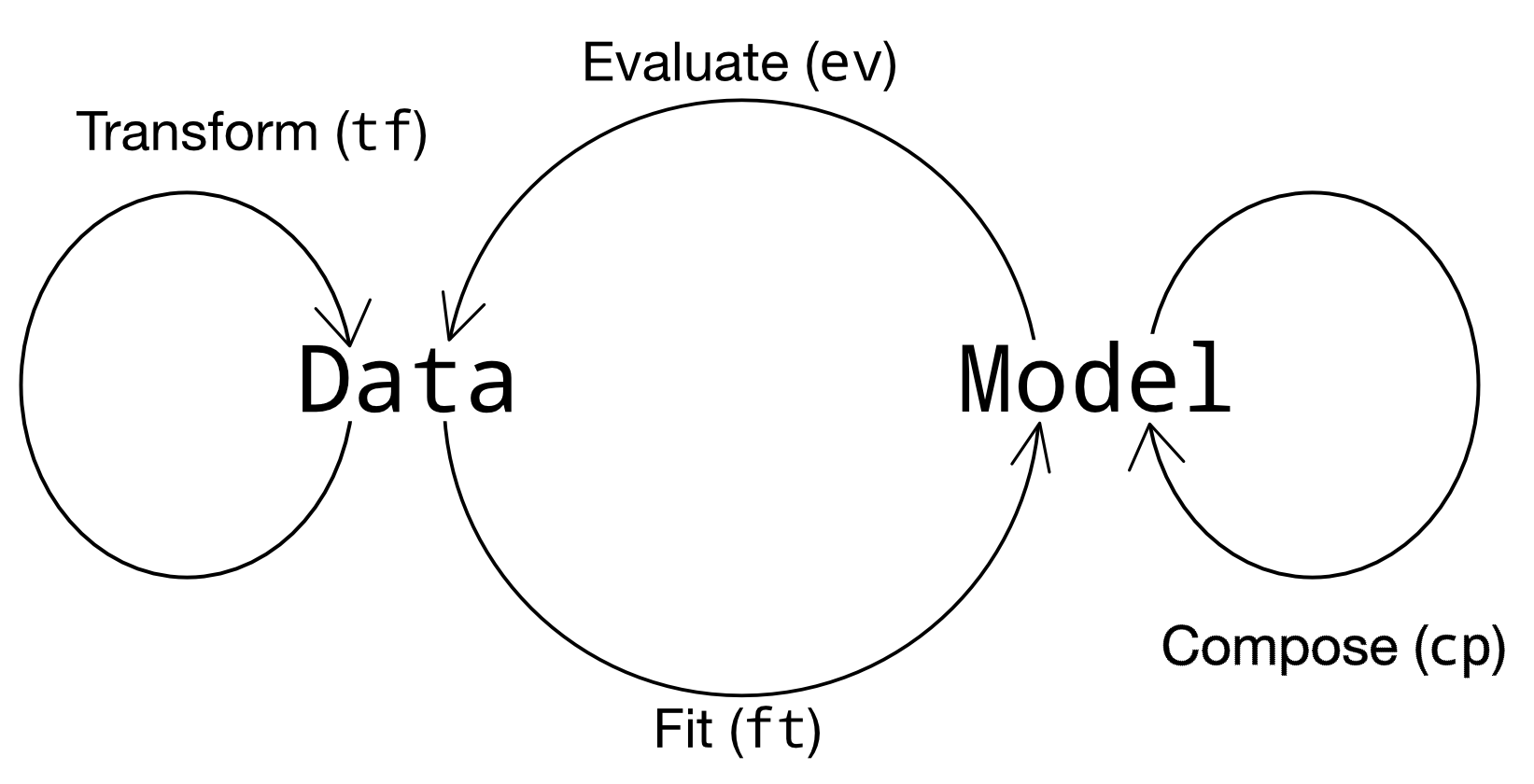
Recall that there are four classes of verb in grama; fitting verbs take data as an input and produce a model as an output. There are various ways to fit a model; in this exercise we’ll focus on fitting a parameterized model using nonlinear least squares.

Grama verb class diagram

Trajectory Data#

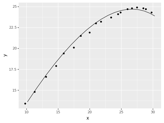
We’re going to use the following trajectory dataset to fit a function predicting the trajectory. Our goal in this case study is as follows:

Our goal is to fit a trajectory model and accurately predict the range of the projectile.

Note that our data only covers the beginning of the trajectory; we can’t see where it lands (hence, we don’t know its range).

# NOTE: No need to edit
from grama.data import df_trajectory_windowed
(
    df_trajectory_windowed
    >> gr.ggplot(gr.aes("x", "y"))
    + gr.geom_point()
)

../_images/d20-e-grama05-fit-function-solution_6_0.png

<ggplot: (8789009847730)>

EMA of Proposed Model#

Before we jump immediately to using statistical procedures to fit a function, let’s first use EMA to understand the model we’re going to fit.

Trajectory model#

The following code loads a model for the trajectory of a projectile subject to a linear drag force.

from grama.models import make_trajectory_linear
md_trajectory = make_trajectory_linear()
md_trajectory

model: Trajectory Model

  inputs:
    var_det:
      u0: [0.1, inf]
      tau: [0.05, inf]
      t: [0, 600]
      v0: [0.1, inf]

    var_rand:

    copula:
      None

  functions:
      x_trajectory: ['u0', 'v0', 'tau', 't'] -> ['x']
      y_trajectory: ['u0', 'v0', 'tau', 't'] -> ['y']

Linear drag model#

The drag \(\vec{F}_d\) acting on the projectile in this model has a magnitude equal to

\[F_d \propto - m \tau s\]

where \(m\) is the mass of the projectile, \(s\) is its speed, and \(\tau\) is the time constant associated with the drag law.

We can make sense of the model by inspecting the equations in the model. However, a complementary way to gain understanding is to do a little exploratory model analysis. You’ll use EMA below to understand the model’s behavior.

Sinews and bounds#

One “gotcha” with ev_sinews() is that it can only sweep inputs with finite bounds. For variables with one-sided bounds, such as [0.1, inf], we cannot sweep values all the way to infinity! Instead, grama will set the inputs with one-sided bounds to their lower bound, and sweep the remaining variables. We need to set finite bounds in order to use gr.ev_sinews().

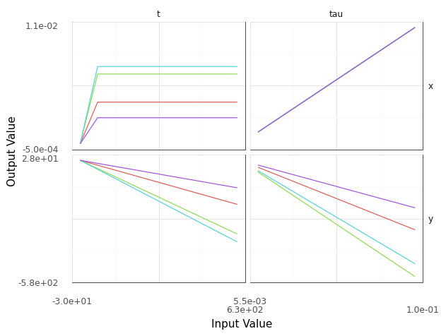
q1 Sweep values of `tau`#

Update the model to enable a sweep over values of tau. How does changing tau affect the trajectory? Answer the questions under observations below.

Hint: Remember that gr.cp_bounds() allows you to adjust the bounds of a grama model. Note that you may need to adjust the bounds of time t as well as tau to make an informative plot.

(
    md_trajectory
    >> gr.cp_bounds(tau=[0.01, 0.1])
    >> gr.ev_sinews(df_det="swp", n_sweeps=4)
    >> gr.pt_auto()
)

Calling plot_sinew_outputs....

/Users/zach/opt/anaconda3/envs/evc/lib/python3.9/site-packages/plotnine/utils.py:371: FutureWarning: The frame.append method is deprecated and will be removed from pandas in a future version. Use pandas.concat instead.

../_images/d20-e-grama05-fit-function-solution_13_2.png

<ggplot: (8788972083167)>

Observations

Once you get a sweep of tau displayed, what do each of the curves in the tau column represent?
- Each curve in the tau column represents the effect tau has on the relevant output (x or y) at a fixed point in time t.
What affect does tau have on the trajectory range x at a fixed point in time t?
- Increasing tau tends to increase the range at a fixed point in time.
What affect does tau have on the trajectory height y at a fixed point in time t?
- Increasing tau tends to decrease the height at a fixed point in time.

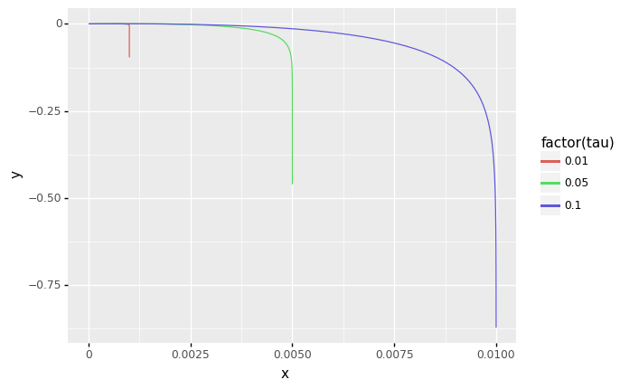
q2 Plot a few trajectories#

Complete the code below to sweep over values of tau and t. Compare these results with what you found above. Answer the questions under observations below.

# TASK: Sweep tau and t to create trajectories
(
    md_trajectory
    >> gr.ev_df(
        df=gr.df_grid(
            u0=0.1,
            v0=0.1,

            tau=[0.01, 0.05, 0.1],
            t=gr.linspace(0, 1, 100)
        )
    )
    >> gr.ggplot(gr.aes("x", "y", color="factor(tau)"))
    + gr.geom_line()
)

../_images/d20-e-grama05-fit-function-solution_16_0.png

<ggplot: (8789009954823)>

Observations

What affect does tau have on the trajectory?
- Increasing tau tends to extend the trajectory, allowing the projectile to reach longer distances.
Imagine that y == 0 represents the ground. Are the endpoints of these trajectories physically reasonable?
- No; the endpoints are below the ground.

Fitting with Least Squares#

Above, we used EMA to make sense of the model’s behavior, but we only guessed at parameter values. Now let’s use a statistical fitting procedure to get reasonable values for the inputs.

The `ft_nls()` routine#

The gr.ft_nls() routine is a fitting routine; it takes in a dataset and returns a (fitted) model. NLS stands for nonlinear least squares, a general-purpose way to fit a parameterized function to a dataset. There is a great deal of statistical theory underpinning NLS, which we will not cover in this exercise. The short version is: NLS seeks input (parameter) values of a function that give the best “agreement” between the function’s output and measured output values.

There are a number of practical concerns to using NLS effectively, which we’ll study below.

q3 Run `ft_nls()`#

Use gr.ft_nls() to fit the model md_trajectory to the data df_trajectory_windowed. Answer the questions under observations below.

Hint: Make sure to read the documentation of an unfamiliar function to learn how to use it!

# TASK: Fit a model to the data
md_fit = (
    df_trajectory_windowed

    >> gr.ft_nls(md=md_trajectory)
)

## NOTE: Use this to check your work
assert \
    isinstance(md_fit, gr.Model), \
    "md_fit is not a model; make sure to fit a model"

md_fit

... fit_nls setting out = ['y', 'x']
... eval_nls setting out = ['y', 'x']
... eval_nls setting var_fix = []
... eval_nls setting var_feat = {'t'}
           u0   tau          v0  u0_0  tau_0  v0_0  success  \
0  425.161431  0.05  447.996569   0.1   0.05   0.1     True   

                                            message  n_iter       mse  
0  CONVERGENCE: NORM_OF_PROJECTED_GRADIENT_<=_PGTOL       3  25.49725  

model: Trajectory Model (Fitted)

  inputs:
    var_det:
      t: (unbounded)

    var_rand:

    copula:
      None

  functions:
      Fix variable levels: ['t'] -> ['u0', 'tau', 'v0']
      Trajectory Model: ['u0', 't', 'tau', 'v0'] -> ['y', 'x']

Observations

The gr.ft_nls() routine should print some diagnostic information; was the optimizer successful in finding best-fit input values? How do you know?
- According to the diagnostics, yes. The success column indicates True.
The gr.ft_nls() starts from an “initial guess” for each of the inputs; these are shown in the diagnostic information as the input names with the suffix _0. What were the initial guess values for the inputs?
- tau_0=0.05, u0_0=0.1, v0_0=0.1

The fitting diagnostics only tell us so much; it is a far better idea to compare predictions from the model directly against the original data.

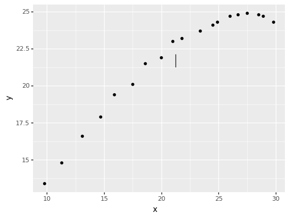
q4 Assess the fit#

Evaluate the fitted model md_fit to compare the predicted values against the original dataset. Answer the questions under observations below.

# TASK: Compare the model predictions with
# the original data df_trajectory_windowed
(
    md_fit

    >> gr.ev_df(df_trajectory_windowed)
    
    >> gr.ggplot(gr.aes("x", "y"))
    + gr.geom_line()
    + gr.geom_point(data=df_trajectory_windowed)
)

... provided columns intersect model output.
eval_df() is dropping {'y', 'x'}

../_images/d20-e-grama05-fit-function-solution_25_1.png

<ggplot: (8788972445868)>

Observations

How well does the fitted model (solid line) agree with the measured values (dots)?
- Terrible! The fitted model somehow gives a small vertical segment in the middle of the plot. This looks nothing like the measured values!

Rough estimation#

Clearly, using completely-arbitrary guesses for the initial parameter values has led to a terrible fit. Let’s do some back-of-the envelope calculations to get a rough sense of reasonable parameter values.

The horizontal velocity is the time-derivative of horizontal position; we can approximate this with a simple finite-difference

\[u = \frac{dx}{dt} \approx \frac{u(t_2) - u(t_1)}{t_2 - t_1}\]

The gr.lead() function allows us to access values in the following row; we can use this to implement differences like \(u(t_2) - u(t_1)\). In code, this would be gr.lead(DF.u) - DF.u.

We can estimate the velocity of the projectile directly using the position and time data, but we’ll have to work a little harder to estimate a reasonable value for tau. To do this, let’s turn to the drag law:

\[F_d \propto - m \tau s\]

Re-arranging to isolate \(\tau\), we find

\[F_d/m/s \propto - \tau\]

\[|a_d / s| \propto |\tau|\]

where \(a_d\) is the acceleration due to drag. Note that this is not the total acceleration! This is just the acceleration due to drag, which we can’t access from the data alone. However, we can use the total acceleration to set a reasonable first-guess for the value of tau.

The following code implements the calculations described above and computes summary statistics over the estimated u, v, tau values.

# NOTE: No need to edit
(
    df_trajectory_windowed
    # Estimate velocity components
    >> gr.tf_mutate(
        u=(gr.lead(DF.x) - DF.x) / (gr.lead(DF.t) - DF.t),
        v=(gr.lead(DF.y) - DF.y) / (gr.lead(DF.t) - DF.t),
    )
    # Compute speed
    >> gr.tf_mutate(s=gr.sqrt(DF.u**2 + DF.v**2))
    # Estimate acceleration
    >> gr.tf_mutate(
        a=(gr.lead(DF.s) - DF.s) / (gr.lead(DF.t) - DF.t)
    )
    # Estimate drag time constant
    >> gr.tf_mutate(tau=gr.abs(DF.a / DF.s))
    
    >> gr.tf_select("u", "v", "tau")
    >> gr.tf_describe()
)

	u	v	tau
count	18.000000	18.000000	17.000000
mean	11.111111	6.055556	4.463891
std	4.114378	6.512181	4.756788
min	4.000000	-4.000000	0.194824
25%	8.250000	1.250000	1.401754
50%	11.000000	4.000000	2.465337
75%	14.750000	12.500000	5.897357
max	18.000000	18.000000	16.172505

This does not directly provide the “best” parameter values for u, v, tau. However, this gets us in the right ballpark. Choosing values similar to the above will be much more effective than picking completely-arbitrary initial guess values.

q5 Choose reasonable initial parameters#

Override the default initial parameter guess of ft_nls() by adding a keyword argument. Using the rough estimates above, you should be able to achieve a fit of the data that is quite reasonable. Answer the questions under observations below.

Hint: Remember to consult the documentation for ft_nls() to see how to use its arguments!

# TASK: Set a reasonable initial guess for the input values
md_fit_init = (
    df_trajectory_windowed
    >> gr.ft_nls(
        md=md_trajectory,
        df_init=gr.df_make(
            u0=18,
            v0=18,
            tau=16,
        )
    )
)

## NOTE: Use this to check your work
(
    md_fit_init
    >> gr.ev_df(df_trajectory_windowed)
    
    >> gr.ggplot(gr.aes("x", "y"))
    + gr.geom_line()
    + gr.geom_point(data=df_trajectory_windowed)
)

... fit_nls setting out = ['y', 'x']
... eval_nls setting out = ['y', 'x']
... eval_nls setting var_fix = []
... eval_nls setting var_feat = {'t'}
          u0       tau         v0  u0_0  tau_0  v0_0  success  \
0  18.792122  2.802267  28.234775    18     16    18     True   

                                           message  n_iter       mse  
0  CONVERGENCE: REL_REDUCTION_OF_F_<=_FACTR*EPSMCH      25  0.093358  
... provided columns intersect model output.
eval_df() is dropping {'y', 'x'}

../_images/d20-e-grama05-fit-function-solution_31_1.png

<ggplot: (8788988651201)>

Observations

How well does the trend fit the data? Is the fit perfect?
- Quite well! Certainly much better than the previous attempt. The fit is not perfect though; there seems to be some “jitter” in the measured values.
How does your initial guess for tau compare with the fitted value? What might account for this?
- My initial guess of tau == 16 is quite a bit larger than the fitted value of tau ~= 2.8. As noted above, we estimated a time constant from the total acceleration, rather than the acceleration solely due to drag.
How does your initial guess for u0 compare with the fitted value? What might account for this?
- My initial guess of u0 == 18 is quite close to the fitted value of u0 ~= 18.79. The fitted value is larger, which makes intuitive sense (drag should slow the projectile), though it’s closer than I might have expected.

Model Assessment#

We have successfully fit a function to data! However, before we start using this model to make predictions, we should carry out some model assessment studies to check that this is a reasonable model. The next few tasks will guide you through some useful assessment techniques.

Quantifying uncertainty#

The gr.ft_nls() routine allows us to quantify the uncertainty in the fitted values by fitting a joint distribution for the inputs. As we saw above, the fit of the function to the data is not perfect; therefore, the noise in the measured values implies we cannot estimate the input values perfectly. Setting uq_method="linpool" in gr.ft_nls() accounts for this by finding a “best-fit” value, but additionally fitting a normal distribution to account for the noise in the outputs.

# NOTE: No need to edit
md_fit_uq = (
    df_trajectory_windowed
    >> gr.ft_nls(
        md=md_trajectory,
        df_init=gr.df_make(
            u0=18,
            v0=18,
            tau=16,
        ),
        ## NOTE: This fits a distribution for the inputs
        uq_method="linpool",
    )
)
md_fit_uq 

... fit_nls setting out = ['y', 'x']
... eval_nls setting out = ['y', 'x']
... eval_nls setting var_fix = []
... eval_nls setting var_feat = {'t'}
          u0       tau         v0  u0_0  tau_0  v0_0  success  \
0  18.792122  2.802267  28.234775    18     16    18     True   

                                           message  n_iter       mse  
0  CONVERGENCE: REL_REDUCTION_OF_F_<=_FACTR*EPSMCH      25  0.093358  
... provided columns intersect model output.
eval_df() is dropping {'y', 'x'}

/Users/zach/Git/py_grama/grama/fit_synonyms.py:152: FutureWarning: Passing a set as an indexer is deprecated and will raise in a future version. Use a list instead.

model: Trajectory Model (Fitted)

  inputs:
    var_det:
      t: (unbounded)

    var_rand:
      u0: (+0) norm, {'mean': '1.879e+01', 's.d.': '1.700e-01', 'COV': 0.01, 'skew.': 0.0, 'kurt.': 3.0}
      tau: (+0) norm, {'mean': '2.800e+00', 's.d.': '1.300e-01', 'COV': 0.05, 'skew.': 0.0, 'kurt.': 3.0}
      v0: (+0) norm, {'mean': '2.823e+01', 's.d.': '2.000e-01', 'COV': 0.01, 'skew.': 0.0, 'kurt.': 3.0}

    copula:
      Gaussian copula with correlations:
  var1 var2      corr
0   u0  tau -0.678984
1   u0   v0  0.000000
2  tau   v0 -0.704758

  functions:
      Trajectory Model: ['u0', 't', 'tau', 'v0'] -> ['y', 'x']

Since this is a grama model, we can use the same kind of sampling tools we’ve seen before to inspect the uncertainty in the fitted input values.

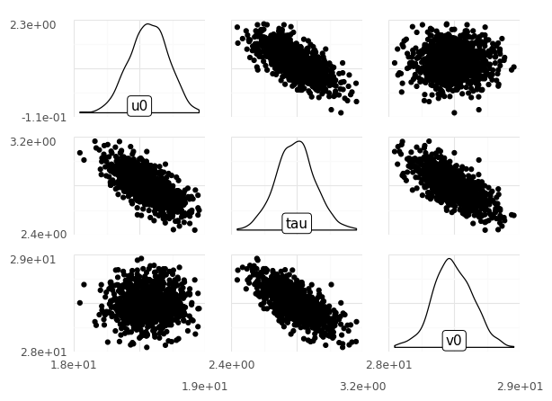
q6 Inspect plausible input values#

The following code visualizes the input uncertainty of the fitted values. Run the code below, and answer the questions under observations below.

# TASK: Run and inspect
(
    md_fit_uq
    >> gr.ev_sample(n=1e3, df_det="nom", skip=True)
    >> gr.pt_auto()
)

eval_sample() is rounding n...
Design runtime estimates unavailable; model has no timing data.
Calling plot_scattermat....

/Users/zach/Git/py_grama/grama/plot_auto.py:234: UserWarning: Matplotlib is currently using module://matplotlib_inline.backend_inline, which is a non-GUI backend, so cannot show the figure.

../_images/d20-e-grama05-fit-function-solution_38_2.png

Observations

How variable are each of the inputs?
- None of the inputs seem that variable; tau ranges between 2.2 and 3.3, u0 between 18 and 19, and v0 between 27 and 29.

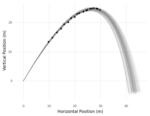
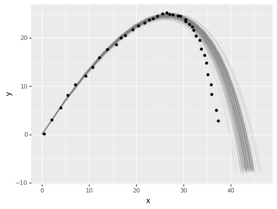
q7 Inspect plausible trajectories#

Draw a random sample of trajectories to study the uncertainty in in the outputs. Make sure to pick a reasonable range of time values t so that you can see both the beginning and end (ground-strike at y==0) of the trajectory. Answer the questions under observations below.

# TASK: Evaluate the model
(
    md_fit_uq

    >> gr.ev_sample(
        n=100, 
        df_det=gr.df_make(t=gr.linspace(0, 4.8, 20))
    )
    
    ## NOTE: No need to edit below here; this will visualize your results
    >> gr.ggplot(gr.aes("x", "y"))
    # NOTE: The `group` aesthetic allows us to draw
    # individual lines for each value of u0; otherwise
    # the lines would all be connected
    + gr.geom_line(gr.aes(group="u0"), alpha=1/5, color="grey")
    # Add the data
    + gr.geom_point(data=df_trajectory_windowed)
    # Clean up the visual
    + gr.theme_minimal()
    + gr.labs(
        x="Horizontal Position (m)",
        y="Vertical Position (m)",
    )
)

../_images/d20-e-grama05-fit-function-solution_41_0.png

<ggplot: (8788988482241)>

Observations

Compare the ensemble of trajectories (grey lines) against the measured values (black dots); is the uncertainty in the trajectory comparable to the observed variability in the measured values? How do you know?
- Yes; the ensemble of trajectories covers a similar “width” as the measured values.
According to the fitted model, what is a plausible final range for the projectile? (In what band of x values does it hit the ground at y == 0?)
- The trajectories in the plot range from around x_range == 40 to x_range = 45.

Model Validation#

One of the most important assessments we should carry out is model validation. When validating a model, we use a dataset that was not used to fit the model in order to check how well the model agrees with physical reality. This is to help avoid the statistical phenomenon of overfitting.

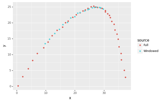
Validation data#

Let’s load a dataset that is appropriate for validation; the following data is from the same trajectory as df_trajectory_windowed, but it consists of independent observations, and it runs for a longer span of time values.

## NOTE: No need to edit
from grama.data import df_trajectory_full
(
    df_trajectory_full
    >> gr.tf_mutate(source="Full")
    >> gr.tf_bind_rows(
        df_trajectory_windowed
        >> gr.tf_mutate(source="Windowed")
    )
    >> gr.ggplot(gr.aes("x", "y", color="source"))
    + gr.geom_point()
)

../_images/d20-e-grama05-fit-function-solution_45_0.png

<ggplot: (8788954606201)>

q8 Compare the fit to validation data#

Compare the predictions from the fitted model md_fit_uq to compare an ensemble of trajectories against the validation data df_trajectory_full. Answer the questions under observations below.

Hint: This part has no starter code! Use what you learned above to carry out this comparison.

# TASK: Compare the fitted model to the validation data;
# make sure to quantify the parameter uncertainty
(
    md_fit_uq
# solution-begin 
    >> gr.ev_sample(
        n=100, 
        df_det=gr.df_make(t=gr.linspace(0, 5, 20))
    )
    
    >> gr.ggplot(gr.aes("x", "y"))
    + gr.geom_line(gr.aes(group="u0"), alpha=1/5, color="grey")
    + gr.geom_point(data=df_trajectory_full)
# solution-end 
)

../_images/d20-e-grama05-fit-function-solution_47_0.png

<ggplot: (8788972613545)>

Observations

How well does the model fit the data? Does the model perform better in some regions than others?
- The model fits well at the beginning of the trajectory, but does progressively worse further into the trajectory. Towards the end, the model overpredicts the range by quite a bit! (A few meters.)

The dramatic reveal…#

It turns out the model does not accurately predict the trajectory’s range! This is because our model assumes a linear drag law \(F_d \propto - m \tau s\), while in reality the data were generated using a quadratic drag law \(F_d \propto - m b s^2\). This qualitative difference between the model and the data-generating process leads to a mismatch between predicted and measured values that we can’t overcome without changing the model’s form.

This is why validation is so important: It is difficult to discover this kind of model form error without a validation study. In practice, data scientists will use a train-validation split to help construct this sort of validation study.

Data Science for Engineers

Grama: Fitting Functions

Contents

Grama: Fitting Functions#

Setup#

Fitting#

Trajectory Data#

EMA of Proposed Model#

Trajectory model#

Linear drag model#

Sinews and bounds#

q1 Sweep values of `tau`#

q2 Plot a few trajectories#

Fitting with Least Squares#

The `ft_nls()` routine#

q3 Run `ft_nls()`#

q4 Assess the fit#

Rough estimation#

q5 Choose reasonable initial parameters#

Model Assessment#

Quantifying uncertainty#

q6 Inspect plausible input values#

q7 Inspect plausible trajectories#

Model Validation#

Validation data#

q8 Compare the fit to validation data#

The dramatic reveal…#

Further Reading#

Data Science for Engineers

Grama: Fitting Functions

Contents

Grama: Fitting Functions#

Setup#

Fitting#

Trajectory Data#

EMA of Proposed Model#

Trajectory model#

Linear drag model#

Sinews and bounds#

q1 Sweep values of tau#

q2 Plot a few trajectories#

Fitting with Least Squares#

The ft_nls() routine#

q3 Run ft_nls()#

q4 Assess the fit#

Rough estimation#

q5 Choose reasonable initial parameters#

Model Assessment#

Quantifying uncertainty#

q6 Inspect plausible input values#

q7 Inspect plausible trajectories#

Model Validation#

Validation data#

q8 Compare the fit to validation data#

The dramatic reveal…#

Further Reading#

q1 Sweep values of `tau`#

The `ft_nls()` routine#

q3 Run `ft_nls()`#