Exercises in Machine Learning¶

Author: Zach del Rosario

The primary purpose of this notebook is to help you not get fooled by machine learning! As Drew Conway notes, possessing hacking skills and substantive experience—but having no math or statistics background—puts one in the danger zone. While we can’t possibly cover everything you need in a single workshop, this exercise will highlight some of the challenges of doing machine learning well. See the Further Reading section at the end for suggestions on learning more.

Learning outcomes¶

By working through this notebook, you will be able to:

Use grama to work with models.
Understand the importance of underfitting and overfitting.
Use cross-validation to help avoid underfitting and overfitting.
State some example ways underfitting and overfitting show up studying a materials dataset.
Use these concepts on a case study with real materials data.

Tips:

This exercise heavily uses the py-grama package; you can find more info on the documentation site.
This exercise indirectly uses scikit-learn; you can find lots of useful info on this package on their documentation site.

# Setup
import numpy as np
import pandas as pd
import grama as gr
%matplotlib inline

DF = gr.Intention()

# Show all pandas columns
pd.set_option("display.max_columns", None)

# For downloading data
import os
import requests

The following code sets up some helper functions that are used throughout the notebook.

# Helper functions
def add_noise(function, sigma=0.1, seed=101):
    """Add noise to deterministic functions
    """
    def new_function(x):
        np.random.seed(seed)
        y = function(x)
        return y + sigma * np.random.normal(size=y.shape)

    return new_function

# Reference points for regression examples
X_ref = np.linspace(-1, +1, num=100)

# Reference models
def fcn_1(x): return (0.3 * x**2 + 1.0 * x + 2)
def fcn_2(x): return (-2.0 * x**3 + 0.4 * x**2 + 1.0 * x + 2)

fcn_1_noisy = gr.make_symbolic(add_noise(fcn_1))
fcn_2_noisy = gr.make_symbolic(add_noise(fcn_2, sigma=0.2))

# Package as a dataframe
df_data = gr.df_make(
    x=X_ref,
    y_1=fcn_1_noisy(X_ref),
    y_2=fcn_2_noisy(X_ref),
)

Regression Helper Function¶

This function will automate some steps so we can focus on high-level ideas, but I define it here in case you’d like to see the details.

## For partial evaluation
from toolz import curry
## Model training tools
from sklearn.linear_model import LinearRegression
from sklearn.preprocessing import PolynomialFeatures

## Encapsulate featurizer and regressor in one object
class FunctionLM(gr.Function):
    def __init__(self, regressor, var, out, name, order, runtime):
        self.regressor = regressor
        self.var = var
        self.out = list(map(lambda s: s + "_mean", out))
        self.name = name
        self.order = order
        self.runtime = runtime

    def eval(self, df):
        ## Check invariant; model inputs must be subset of df columns
        if not set(self.var).issubset(set(df.columns)):
            raise ValueError(
                "Model function `{}` var not a subset of given columns".format(
                    self.name
                )
            )

        ## Featurize
        x = np.atleast_2d(df[self.var].values)
        poly = PolynomialFeatures(self.order)
        X_feat = poly.fit_transform(x)
        
        ## Predict
        y = self.regressor.predict(X_feat).flatten()
        return pd.DataFrame(data=y, columns=self.out)

## Fitting routine
@curry
def fit_regression(df, var=None, out=None, order=1):
    r"""Fit a linear regression of specified order
    
    Args:
        df (DataFrame): Data for fitting
        var (iterable of str): Names of input variable (feature); must be column in df
        out (iterable of str): Name of output variable (response); must be column in df
        order (int): Polynomial order for fit
    
    """
    if len(out) > 1:
        raise ValueError("This simple helper can only handle one output.")
    # Featurize
    x = np.atleast_2d(df[var].values)
    poly = PolynomialFeatures(order)
    X_feat = poly.fit_transform(x)
    
    # Fit regression
    y = np.atleast_2d(df[out].values)
    lm = LinearRegression()
    lm.fit(X_feat, y)
    
    # Package
    fun = FunctionLM(lm, var, out, "Linear Model", order, 0)
    
    return gr.Model(functions=[fun], domain=None, density=None)
    
## Create pipe-enabled regression utility
ft_regression = gr.add_pipe(fit_regression)

Underfitting and Overfitting¶

First we’ll cover some key ideas on simple cases. These are not ‘real’ data, but the simplicity of the examples will allow us to focus on concepts.

Here I generate some data from a simple polynomial.

## NOTE: No need to edit
# Ground-truth data; no noise
df_ex1 = (
    gr.df_make(x=np.linspace(-1, +1, num=10))
    >> gr.tf_mutate(y=fcn_1(DF.x))
)

# Plot
(
    df_ex1
    >> gr.ggplot(gr.aes("x", "y"))
    + gr.geom_point()
)

We will fit a simple linear regression to these data. To do this, we’ll use the linear regression helper ft_regression() (defined above). To start, we’ll assume that the data were generated from an underlying rule (a model) of the form

\[y_{\text{mean}} = m x + b,\]

and attempt to learn the slope \(m\) and intercept \(b\) by minimizing the difference between the measured values y and the predicted values y_mean.

## NOTE: No need to edit
# Fit the line
md_line = (
    df_ex1
    >> ft_regression(var=["x"], out=["y"], order=1)
)

# Predict
df_line_pred = (
    md_line
    >> gr.ev_df(df=df_ex1)
)

# Plot results
(
    df_line_pred
    >> gr.ggplot(gr.aes("x", "y_mean"))
    + gr.geom_line(linetype="dashed", color="grey")
    + gr.geom_point(color="grey")
    + gr.geom_point(gr.aes(y="y"))
)

The ft_regression() tool returns a grama model; let’s learn about this toolset.

Working with models in Grama¶

In addition to the data transformation tools we used in previous notebooks, grama provides a model object to simplify working with different forms of model. The grama documentation has more information, but let’s focus on the high-level details.

Like with a DataFrame, we can get a view of the model simply by printing it out:

## NOTE: No need to edit, run to show info on `md_line`
md_line

The text above is a summary of what’s in the model. Based on this summary, we can see that it takes a single input x and maps it to a single output y_mean. This can be particularly useful for checking the “basic facts” about the model: what inputs does it require? What outputs does it provide?

Note that we fit a model to predict an output y, but our model provides y_mean. This renaming is deliberate; we’re providing a predicted value, not a measured value. Since our model is based on a statistical mean, the output gets the _mean suffix.

One of the most important uses of a fitted model is to predict unobserved output values. We can do this with a grama model by providing values for the desired inputs and evaluating the model.

Q1: Evaluate the model at new input values¶

Use the function gr.ev_df() to evaluate the model md_line fitted above. Make use of the new set of input values df_dense. Answer the questions below.

###
# TASK: Evaluate md_line at the df_dense input values.
###

# -- FINISH THE CODE BELOW -----
df_dense = gr.df_make(x=np.linspace(-1, +1, num=100))

df_evaluated = (
    md_line
## TODO: Evaluate the model here

)

# -- NO NEED TO EDIT BELOW HERE -----
(
    df_evaluated
    >> gr.tf_mutate(source="Fit")
    >> gr.ggplot(gr.aes("x", "y_mean", color="source"))
    + gr.geom_line(linetype="dashed")
    + gr.geom_point()
    + gr.geom_point(
        data=df_ex1
        >> gr.tf_mutate(source="Measured"),
        mapping=gr.aes(y="y"),
    )
)

Observe

How many points are measured? How many are fit? (Note: Don’t count by hand, try looking at the code!)
- (Your response here)
Suppose we wanted to evaluate the quality of our fit. At how many locations could we evaluate the quality of the fit? Why?
- (Your response here)

Model Flexibility and Underfitting¶

Note that we had to assume a model-form in order to do the fitting: \(y_{\text{mean}} = m x + b\). From the figure above, we can see that the model is close to the true values, but obviously lacks the curvature of the true data-generating process.

This phenomenon—the failure of a model to capture behavior in the data—is called underfitting. To reduce underfitting, we need to make our model more flexible. For a linear regression, we can do this by increasing the order of the regression.

Q2: Fit a quadratic model to the data¶

Use the ft_regression() helper to fit a quadratic model (order = 2).

###
# TASK: Fit a quadratic model
###

# -- FINISH THE CODE BELOW -----
# Fit a quadratic
md_quad = (
    df_ex1
## TODO: Fit a regression here

)

# -- NO NEED TO EDIT BELOW HERE -----
# Predict
df_quad_pred = (
    md_quad
    >> gr.ev_df(df=df_ex1)
)

# Plot results
(
    df_quad_pred
    >> gr.ggplot(gr.aes("x", "y_mean"))
    + gr.geom_line(linetype="dashed")
    + gr.geom_point(gr.aes(y="y"))
)

Here we can see the model fits the data perfectly. This suggests that we have successfully discovered the exact rule that generated these data, which in this special case happens to be true.

However, we will very rarely be able to fit the true function exactly. This is because real data tend to have noise, which corrupts the underlying function we are trying to learn.

Noise and Overfitting¶

Below, I generate data from the same model, but add a little bit of noise.

## NOTE: No need to edit
# Ground-truth data; now with noise
df_ex2 = (
    gr.df_make(x=np.linspace(-1, +1, num=10))
    >> gr.tf_mutate(y=fcn_1_noisy(DF.x))
)

# Plot
(
    df_ex2
    >> gr.ggplot(gr.aes("x", "y"))
    + gr.geom_point()
)

Let’s see what happens when we fit a quadratic to the noisy data.

## NOTE: No need to edit
(
    df_ex2
    >> ft_regression(var=["x"], out=["y"], order=2)
    >> gr.ev_df(df=df_ex2)
    
    >> gr.ggplot(gr.aes("x", "y_mean"))
    + gr.geom_line(linetype="dashed")
    + gr.geom_point(gr.aes(y="y"))
)

Here we can see that the fit is no longer perfect, despite coming from the “same” model. Since we already know that a quadratic can fit the underlying function perfectly, underfitting is not the issue here. Instead, the error is increased due to the noise in the data.

However, we have not yet seen a case of overfitting. To see that phenomenon, let’s keep increasing the order of the model.

Q3: Overfit the model¶

Increase the order of the regression until the model goes through every measured point. Does this seem like a reasonable model?

###
# TASK: Increase the order until the fit is perfect
###

# -- FINISH THE CODE BELOW -----
(
    df_ex2
    >> ft_regression(
        var=["x"], 
        out=["y"], 
        order=2 # TODO: Increase the order until the fit is perfect
    )
    >> gr.ev_df(df=gr.df_make(x=np.linspace(-1, +1, num=100)))
    
    >> gr.ggplot(gr.aes("x", "y_mean"))
    + gr.geom_line(linetype="dashed")
    + gr.geom_point(
        data=df_ex2,
        mapping=gr.aes(y="y"),
    )
)

Balancing Overfitting and Underfitting¶

To help illustrate, let’s look at one more synthetic example

## NOTE: No need to edit
# More complicated function with noise
df_ex3 = (
    gr.df_make(x=np.linspace(-1, +1, num=10))
    >> gr.tf_mutate(y=fcn_2_noisy(DF.x))
)

(
    df_ex3
    >> gr.ggplot(gr.aes("x", "y"))
    + gr.geom_point()
)

Here we can see a somewhat complicated function that is quite corrupted by noise. Below, I’m going to fit a number of polynomial models of different orders. In practice, we would like to make a decision about what polynomial order to use. A sensible choice would be to pick the order that minimizes the error—let’s see which model accomplishes this.

# -- DEMONSTRATION CODE, NO NEED TO EDIT -----
# Fit on many different orders
df_train_err = pd.DataFrame()
df_test_err = pd.DataFrame()
for order in range(1, 10):
    # Fit the model
    md_tmp = (
        df_ex3
        >> ft_regression(var=["x"], out=["y"], order=order)
    )
    # Evaluate model on training data
    df_tmp = (
        md_tmp
        >> gr.ev_df(df=df_ex3)
        >> gr.tf_mutate(order=order)
    )
    df_train_err = pd.concat((df_train_err, df_tmp), axis=0)
    # Evaluate model on test data
    df_tmp = (
        gr.df_make(x=np.linspace(-1, +1, num=100))
        >> gr.tf_mutate(y=fcn_2(DF.x), order=order)
        >> gr.tf_md(md=md_tmp)
    )
    df_test_err = pd.concat((df_test_err, df_tmp), axis=0)

# Visualize a few cases
(
    df_train_err
    >> gr.tf_filter(gr.var_in(DF.order, [1, 3, 9]))
    >> gr.ggplot(gr.aes("x", "y_mean"))
    + gr.geom_line(gr.aes(color="factor(order)"), linetype="dashed")
    + gr.geom_point(data=df_ex3, mapping=gr.aes(y="y"))
)

Here I’ve selected just a few of the models to plot. We can see

The Order = 1 case is underfit, like we saw in the example above
The Order = 9 case curves tortuously to go through many points; this is an example of overfitting
The Order = 3 case is not perfect, but tends to balance between underfitting and overfitting. This is a well-fit model.

More generally, overfitting is when the model fits to spurrious patterns in the data; essentially, we are fitting to noise, rather than signal. We would like to detect and avoid overfitting in practice! While we can see above some suspicious behavior based on the fitted curves, we might like a quantitative way to compare models; in particular, once we have multiple inputs we won’t be able to create simple y vs x plots like we do above.

Additionally, there’s a subtle issue that we’ll run into when it comes to evaluating the accuracy of a model: The Order = 9 case clearly looks unstable and untrustworthy, but note that the model is perfect at the points where we have measured output values. This is going to present some issues that we’ll see below:

Quantifying Error and Cross-Validating¶

There are a wide variety of ways to quantify the accuracy of a model: The code below computes three example metrics.

## NOTE: No need to edit
(
    df_train_err
    >> gr.tf_group_by(DF.order)
    >> gr.tf_summarize(
        mse=gr.rmse(DF.y_mean, DF.y),
        ndme=gr.ndme(DF.y_mean, DF.y),
        rsq=gr.rsq(DF.y_mean, DF.y),
    )
)

mse is mean-squared error, a common error metric often used in the machine learning community. Smaller values are more accurate.
ndme stands for non-dimensional model error. As the name implies, this quantity is dimensionless, and takes a value of 0 when the model is perfect, and a value of 1 (sometimes higher) when the model is uninformative. This metric is not terribly common, but it is very useful as a dimensionless metric for error.
rsq is short for \(R^2\) (r-squared), also called the coefficient of determination, a common goodness of fit metric used in the statistics community. Higher values are more accurate, with \(R^2 = 1\) indicating a perfect fit.

Train vs Test¶

Remember above how the order = 9 model looked untrustworthy, but went through all of our observed data points? Let’s quantify the error both on the available data (the train data), but check the model’s behavior on an independent set of observations (the test data). The code below plots error estimated using these two different sets of data.

## NOTE: No need to edit
(
    df_train_err
    >> gr.tf_mutate(source="train")
    >> gr.tf_bind_rows(
        df_test_err
        >> gr.tf_mutate(source="test")
    )
    >> gr.tf_group_by(DF.order, DF.source)
    >> gr.tf_summarize(ndme=gr.ndme(DF.y_mean, DF.y))
    
    >> gr.ggplot(gr.aes("order", "ndme"))
    + gr.geom_line(gr.aes(linetype="source"))
    + gr.scale_y_log10()
    + gr.labs(
        x="Polynomial Order",
        y="NDME",
    )
)

Here we can see the train and test error values greatly diverge. This is highly problematic for two interrelated reasons:

In practice, we would only have access to the train curve, as the test curve relies on extra data (that we don’t have).
If we were to make a decision about Polynomial Order based on the train curve, we would choose a much higher order than what would minimize the NDME in the True case.

The underlying reason for the poor error estimate here is that we are using the same data to both train and test the model. We can improve our estimates for the error through various techniques; below, we will use the technique of cross-validation.

Avoiding Optimistic Estimates: Cross-Validation¶

Cross-validation is one technique for estimating the error in a way that avoids the “optimism” we saw above. For the variant k-fold cross-validation (k-fold CV), we split all our data into folds, and use these to build training and test sets. Generally:

Training data are used to fit a model
Test data are used to evaluate a model

CV schematic

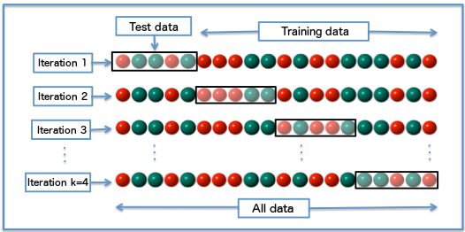
(Schematic for k-fold CV. Fabian Flock, via Wikimedia)

In each of our \(k\) iterations, we do not allow the model to see a test fold (Test data above) during training, and fit the model only on the remaining data (Training data above). After training, we compute our chosen error metric on the test fold. Finally, we repeat this process on each of the \(k\) chosen folds. This gives us a set of less optimistic estimates for the error, which we can summarize e.g. as a mean CV error.

This procedure is implemented in the grama function tf_kfolds(), as demonstrated below. Note that tf_kfolds() takes in a dataset to use for k-fold cross validation, as well as a fitting procedure that we will use for each iteration. The routine also provides some reasonable default values for the number of folds k and the error metrics to compute. We can override these by providing keyword arguments (as you’ll do below).

## NOTE: No need to edit
(
    df_ex3
    >> gr.tf_kfolds(
        ft=ft_regression(var=["x"], out=["y"], order=9),
#         summaries=dict(mse=gr.mse), # Uncomment to override defaults
#         k=3,
    )
)

Note that the k-fold CV estimated rsq_y values are abysmal; they take negative values, which indicates that the model performance is quite bad.

One powerful use of k-fold CV is to do a hyperparameter study: In our case, we’ll study how the model accuracy changes as we sweep over the polynomial order.

Q4: Override the defaults¶

Complete the code below by overriding the default settings for tf_kfolds(). Provide an estimate of the non-dimensional model error (gr.ndme). You can also try changing the value of k to see how the results change.

Answer the questions under Observations below.

Hint: You may find that the code throws errors for larger values of k. Think about how many data points you have available in df_ex3. How many folds can you split the data into while having more than just one point in each fold?

###
# TASK: Increase the order until the fit is perfect
###

# -- FINISH THE CODE BELOW -----
# Fit on many different orders
df_kfolds = pd.DataFrame()
# Iterate over a selection of polynomial orders
for order in range(1, 10):
    # Evaluate model with k-fold CV
    df_tmp = (
        df_ex3
        >> gr.tf_kfolds(
            # Use the desired polynomial order for this iteration
            ft=ft_regression(var=["x"], out=["y"], order=order),
            ## TODO: Override the defaults in tf_kfolds

        )
        # Record the order used in fitting
        >> gr.tf_mutate(order=order)
    )
    # Record the results for this polynomial order
    df_kfolds = pd.concat((df_kfolds, df_tmp), axis=0)
    
# Visualize
(
    df_kfolds
    >> gr.ggplot(gr.aes("order", "ndme_y"))
    + gr.geom_boxplot(gr.aes(group="order"))
    + gr.scale_x_continuous(breaks=range(1, 10))
    + gr.scale_y_log10()
)

Observe

How much do the results change as you change k?
- (Your response here)
What polynomial order would you select, based on the k-fold CV results? Why?
- (Your response here)
Inspect the function definition of fcn_2 at the top of this notebook. What is the true polynomial order of the underlying function?
- (Your response here)

Here we have just one tunable knob (polynomial order) that defines our model. More generally, these kinds of user-selected quantities are called hyperparameters. Cross-validation and related techniques are key to tuning hyperparameters, and generally making choices about what sort of model we ought to choose.

Terminology Alert

Across various communities, the terms “train”, “test”, and “validation” data are used somewhat inconsistently. The term “train” is used most consistently: The training data is a subset of data used to fit the model. However different authors use the terms “test” and “validation” interchangeably.

What’s truly important is that you keep in mind the purpose of data subsets: Which subset is being used to fit the model? (Train) Which subset is being used to estimate error for hyperparameter tuning? (Test or Validation) Do you have a third disjoint subset to give an unbiased error estimate? (Validation or Test). For more information, see the relevant Wikipedia article.

Case Study: Steel Fatigue Strength Prediction¶

So far, we’ve looked at fairly artificial modeling problems. To help illustrate these fitting and cross-validation ideas in a real materials problem, let’s look at predicting the fatigue strength of steel alloys.

The data for this case study come from Agrawal et al. (2014) IMMI.

# Filename for local data
filename_data = "./data/agrawal_data.csv"

# The following code downloads the data, or (after downloaded)
# loads the data from a cached CSV on your machine
if not os.path.exists(filename_data):
    # Make request for data
    url_data = "https://raw.githubusercontent.com/zdelrosario/mi101/main/mi101/data/agrawal_data.csv"
    r = requests.get(url_data, allow_redirects=True)
    open(filename_data, 'wb').write(r.content)
    print("   Alloy data downloaded from public GitHub file")
else:
    # Note data already exists
    print("    Alloy data loaded locally")
    
# Read the data into memory
df_raw = pd.read_csv(filename_data)

# Drop the index columns
df_fatigue_data = (
    df_raw
    >> gr.tf_drop("Unnamed: 0", "Sample Number")
    >> gr.tf_select("Fatigue Strength", "chemical_formula", gr.everything())
)

As always, we start by doing basic checks on the dataset.

## NOTE: No need to edit
df_fatigue_data

We have the outcome column that we seek to model (Fatigue Strength, at \(10^7\) cycles), the chemical composition of the alloy in string-form, and a large number of processing characteristics.

We can inspect a histogram of the fatigue strength to get a sense for the variation in the quantity we seek to model:

(
    df_fatigue_data
    >> gr.ggplot(gr.aes("Fatigue Strength"))
    + gr.geom_histogram(bins=60)
    + gr.theme_minimal()
)

The fatigue strength is highly variable, with a large bulk around 500, but values as low as 250 and over 1000 as well.

NB I had difficulty finding the units for the reported Fatigue Strength in the original publication. Presumably these values are given in MPa.

This dataset has many columns; for modeling our first job should be to sort out what we want to predict, and which columns (features) we should use to predict that quantity. Our linear regression implementation can only handle numeric columns, so let’s inspect the datatypes to see which features our model can handle:

df_fatigue_data.dtypes

The majority of the columns are numeric, except for the chemical_formula. To start, let’s try modeling the strength without any composition information. The following code creates python lists to target the desired response (col_response) and non-composition features (col_features).

## NOTE: Obtain column names for the response and features
col_response = ["Fatigue Strength"]
col_processing = (
    df_fatigue_data
    >> gr.tf_drop(col_response, "chemical_formula")
).columns

col_processing

Q5: Fit a regression to predict the fatigue strength¶

Use the ft_regression() helper to fit a regression (with 1st order) to predict the fatigue strength.

Answer the questions under Observations below.

###
# TASK: Complete the code below to fit a 1st order regression
#       use col_processing as the inputs (var)
#       use col_response as the output (out)
###

# -- FINISH THE CODE BELOW -----
## TODO: Fit a model here
md_fatigue = (

)

# -- NO NEED TO EDIT BELOW -----
(
    md_fatigue
    >> gr.ev_df(df_fatigue_data)
    >> gr.tf_summarize(
        rmse=gr.rmse(DF["Fatigue Strength_mean"], DF["Fatigue Strength"]),
        rsq=gr.rsq(DF["Fatigue Strength_mean"], DF["Fatigue Strength"]),
        ndme=gr.ndme(DF["Fatigue Strength_mean"], DF["Fatigue Strength"]),
    )
)

Observations

How accurate is your model?
- (Your response here)
Is the model flexible enough to accurately capture the behavior in the data?
- (Your response here)
Is the way we’ve estimated error here appropriate for making decisions about the model’s design? E.g. could we reasonably tune the polynomial order with this error estimate?
- (Your response here)

A different kind of flexibility: Featurization¶

What if we wanted to use the chemical composition as a feature? We can’t use the string as it is (what would \(m \times \text{string}\) mean?). Instead, we can go through a process of featurization (also called feature engineering) to create usable numeric columns that our model can use as inputs.

Featurization is a big topic, one that is inherently problem-specific. To get us started, we’re going to use a featurization scheme by Ward et al. (2016), as-implemented in the matminer python package.

The following code applies the featurizer to our chemical formula column.

## NOTE: No need to edit; featurize with the "magpie" featurizer
df_fatigue_magpie = (
    df_fatigue_data
    >> gr.tf_feat_composition(var_formula="chemical_formula")
)

(
    df_fatigue_magpie
    >> gr.tf_select(gr.contains("Magpie"), gr.everything())
)

Note that we now have over 100 new columns derived from the chemical formula. The following code picks feature columns by dropping the response column and string formula.

## Obtain full feature set
col_feat_both = (
    df_fatigue_magpie
    >> gr.tf_drop(col_response, "chemical_formula")
).columns

col_feat_magpie = (
    df_fatigue_magpie
    >> gr.tf_select(gr.contains("Magpie"))
).columns

col_feat_magpie

Q6: Interpret the following results¶

The following code estimates model accuracy both with and without the Magpie (composition) features. Compare the results and answer the questions under Observations below.

## NOTE: No need to edit; run and answer the questions below
df_err_processing = (
    df_fatigue_data
    >> gr.tf_kfolds(
        ft=ft_regression(var=col_processing, out=col_response),
        summaries=dict(ndme=gr.ndme),
        seed=101,
        k=5,
    )
    >> gr.tf_mutate(feats="processing only")
)

df_err_magpie = (
    df_fatigue_magpie
    >> gr.tf_kfolds(
        ft=ft_regression(var=col_feat_magpie, out=col_response),
        summaries=dict(ndme=gr.ndme),
        seed=101,
        k=5,
    )
    >> gr.tf_mutate(feats="Magpie only")
)

df_err_both = (
    df_fatigue_magpie
    >> gr.tf_kfolds(
        ft=ft_regression(var=col_feat_both, out=col_response),
        summaries=dict(ndme=gr.ndme),
        seed=101,
        k=5,
    )
    >> gr.tf_mutate(feats="processing + Magpie")
)

(
    df_err_processing
    >> gr.tf_bind_rows(df_err_magpie)
    >> gr.tf_bind_rows(df_err_both)
    
    >> gr.ggplot(gr.aes("feats", "ndme_Fatigue Strength"))
    + gr.geom_boxplot(gr.aes(group="feats"))
    + gr.scale_y_continuous(limits=[0, 1])
)

Observations:

Which feature set tends to produce a more accurate model?
- (Your response here)
How large is the difference in accuracy between the cases?
- (Your response here)
How important does the chemical composition (as expressed by Magpie features) tend to be in this case study?
- (Your response here)

Conclusion¶

And that’s it! One could certainly take this case study further (hint: it would be interesting to see how different the alloys are in composition…), but hopefully this already gives you a sense for the kinds of investigations you can do in materials informatics.

Materials Informatics 101

Exercises in Machine Learning

Contents