Intro to Python and Jupyter Notebooks

Intro to Python and Jupyter Notebooks¶

Original Authors: Enze Chen, Malcolm Davidson, Zach del Rosario

This notebook introduces some of the most important features of Jupyter notebooks and some handy tips to keep in mind.

Learning outcomes¶

Throughout this workshop, we will be totally upfront about what precisely we want to you to learn how to do. This learning outcomes section in each notebook will list our objectives. By working through this notebook, you will be able to:

Use basic Jupyter notebook organization and functions.
Create and execute Code cells.
Use basic Python concepts: variables, packages, loops, and conditionals

Highest-level View¶

Throughout this day of the workshop, we will be writing computer software. Before diving into the details, it is beneficial to understand what tools we’ll be using, and why.

Python¶

Python is a programming language, and an extremely popular one at that. Python is praised for its readability, is consistently ranked as a top programming language, and is used by both top software companies and scientists doing computation. All of this is to say that knowing how to write Python code is a valuable skill.

Jupyter¶

Jupyter is a programming environment, often used for writing and sharing Python code. Just as one could choose to write English on stone tablets or on paper, one could choose to write Python code in simple files or in jupyter notebooks. These notebooks are useful for a number of reasons:

Multimedia: This document you’re reading now is a jupyter notebook – it is a combination of (executable) Python code and (formatted) plain text. By allowing the juxtaposition of different media (code and natural language, to name a couple options), one can provide human-readable context next to executable software.
Saves state: Jupyter notebooks save state, allowing you to run some code, save the results, close the document and come back to it later. This is certainly possible in other coding environments, but jupyter has built-in facilities to make this easy.
Reproducible: Reproducibility is a critical issue in science – results cannot be considered scientifically valid unless they can be reproduced under similar conditions. The same principles apply to computational experiments; all too often software is written under time pressure, resulting in scattered documentation and analysis. Consolidating documentation and analysis within a single notebook facilitates scientific reproducibility.

Jupyter notebooks are not always the best media for writing code; for instance, python packages are not written in jupyter notebooks. However, for our purposes, jupyter is a good solution.

How to use this Notebook¶

This jupyter notebook is an interactive exercise – it contains some reading, but the focus is on fill-in-the-blank sections that are meant to test your understanding and spark further learning. Pedagogy research shows that so-called active learning – learning by doing – is far more effective than lecture alone. Thus, you will get the most out of this workshop if you do the work! Try – to the best of your ability – to complete the exercises in these notebooks, and please feel free to ask the TA’s questions if you get stuck. (It’s what we’re here for.)

Run this notebook locally!

If you’re reading this on the workshop website—and not in your local jupyter reader—then it is necessary that you download this notebook locally and open it in jupyter. Look for the download bar in the top-right of this page, as pictured below.

download bar

The rightmost button will let you download this page as a jupyter notebook so you can edit it and complete the exercises. See the relevant setup page for more instructions on working in jupyter.

Exercise portions of the notebook will be marked with a “Q” subheading, like the following:

Q0: An example question¶

Here’s an example of an exercise prompt. Follow the directions here to start the exercise.

Jupyter Introduction¶

Cells¶

A Jupyter notebook is organized as a sequence of different cells. Cells contain chunks of information and allow you to switch between text and code.

Current cell: The currently-selected cell will have a color bar appear on the far left. Use your cursor or arrow keys to select different cells.

Create new cell: To create a new cell, click the “+” icon at the top. This will create a cell below the currently selected cell.

Delete a cell: To delete the currently-selected cell, click the “scissors” icon at the top.

Q1: Create a new cell¶

Create a new cell below this one. Note that it has a different background color! This is because cells have different types.

Types of cells¶

There are two types of cells we will discuss here: Markdown and Code. A single cell can only have 1 type.

Markdown: These are text cells that use the Markdown language for formatting. You can put instructions, headings, links, images, and much more; even \(\LaTeX\) (a language for typesetting mathematics). Here is a cheatsheet for Markdown syntax.

Code: These are cells where you can type Python code, just as you would in a .py file. They will have a label In [ ]: to their left.

To switch the type of cell, you can use the dropdown menu at the top of the cell. (Note: While you’re moused-over this cell, the dropdown menu should read Markdown.)

Edit and format / execute cells¶

To edit a Markdown cell, triple-click within the cell if you currently see a blue bar. The color bar on the left will turn green. Then type and edit as normal.

To format (“execute”) a Markdown cell, press Ctrl+Enter when in “edit” mode. The color bar on the left will turn blue and the cursor will disappear. Your formatting will also take effect.

To edit a Code cell, click within the cell. The color bar on the left will turn green. Then type and edit as normal.

To execute a Code cell, press Ctrl+Enter while it is selected. The color bar on the left will turn blue and the cursor will disappear.

Code cells¶

So far we’ve only seen Markdown cells. Let’s see what we can do with Code cells! Try selecting the code cell below this one and executing it.

# This is a python code cell
6 * 7

Note that code cells are visually distinct from markdown cells – they have a grey background and the [-]: prefix.

Python Introduction¶

Simple operations¶

We can use python like a calculator to carry out simple operations. Some of these include:

Simple math operators (+, -, *, /)
Other math operators; exponentiation 10 ** 2 == 100; modulus 3 % 2 == 1
Parentheses (, ) for grouping operations
Python functions; console output print("Hello")

Q2: Average some values¶

Use basic python operations to average the following numbers: [2, 4, 6, 8].

###
# TASK: Average the numbers [2, 4, 6, 8]
# TODO: Use basic python operations to compute the arithmetic mean
###

# -- WRITE YOUR CODE HERE -----

Variables¶

Jupyter notebooks will save variables across different cells. We can assign values with the = operator. Furthermore, typing just the variable on the last line of a code cell will typically display the variable’s values/attributes.

a = 1
b = 2
c = a * b

Q3: Display a variable¶

Display the value of c in the chunk below.

###
# TASK: Display a variable
# TODO: Type the variable name below and execute
###

A couple things happened here. First, the variable was saved. Second, Jupyter notebooks will display the value of any lone variables in the last line of each Code cell. This is helpful for debugging.

If you want to display multiple quantities from a single cell, you can always use a print statement print(variable). For instance, we could write

print(a)
print(b)
print(c)

You can also see that Code cells with output will have an associated Out [#] right below. Notice what happens to the cell below when the code is running.

Lists¶

A list is a Python data structure. We’ll use lists (and other iterable data structures) quite a bit when doing data analysis – generally we have many observations (elements) to consider.

Lists (i.e. arrays) in Python are created with square brackets. The entries of a list are called elements.

l = [1, 2, 3]

The append() method adds a single element to the end of the array. Note how we can add elements of different types to the same list (unlike Java or C++).

l = [1, 2, 3]
l.append("a")
l

Note that I needed to place l at the end of the cell to display the result. append() modified the list in place – it makes the list longer.

We can also combine lists with the + operator.

[1, 2, 3] + [4, 5, 6]

Note that I did not need to write an additional line to print the result. This is because the + operator returns a list as a result, which is printed by jupyter.

Q4: Working with lists¶

Test your understanding of lists; make a prediction about what the following code will display:

list_a = [1, 2, 3]
list_b = [4, 5, 6]
print(list_a + list_b)
print(list_a.append(list_b))

After you’ve made a prediction, make a new cell and test your prediction.

Indexing and Slicing¶

We can access specific elements of a list (and other iterables) by indexing. Python is uses zero-based indexing, meaning the first element of an iterable is 0, the second is 1, and so on.

Index    0    1    2    3    4
List  [ "a", "b", "c", "d", "e" ]

For instance:

l = ["a", "b", "c"]
print("l[0] = {}".format(l[0]))
print("l[1] = {}".format(l[1]))
print("l[2] = {}".format(l[2]))

We can also use negative indices to conveniently access from the “right”.

print("l[-1] = {}".format(l[-1]))
print("l[-2] = {}".format(l[-2]))

In Python, it’s easy to take subsets of lists and strings (i.e. substrings) using slicing. Given a list (string) named var, we can take a subset of elements (characters) ranging from low to high-1 with the syntax var[low:high]. Run the following code and observe what happens.

var = [0, 1, 2, 3, 4, 5]
# var = '012345'
print('The second element:', var[1])
print('The second and third elements:', var[1:3])
print('The second element onwards:', var[1:])
print('Everything before the second element:', var[:1])
print('Everything before the second TO LAST element:', var[:-2])

Q5: Take the middle¶

Using your understanding of python indexing & slicing, select the middle three elements of the following list.

###
# TASK: Take the middle values
# TODO: Use python slicing to take the middle three values
###
test = [-2, -1, 0, +1, +2]

# -- WRITE YOUR CODE BELOW -----

Modules¶

By default, python provides a relatively small set of functionality. To carry out more specialized operations, we can import module. A module is a set of tools that help us carry out some tasks. For instance, the following module will help us control the execution of python code.

# Import a module first
from time import sleep

# Pause code execution for 5 seconds
sleep(5)

# Print some output to signal code has reached this point
print('Cell is finished running!')

In the first line of the above Code cell, we imported a function sleep() from a module. A function takes some number of inputs (possibly zero, like sleep()), and returns some number of outputs (possibly zero, like sleep()). The inputs to a function are called arguments, and are put inside the parentheses, if needed.

Python modules, even when installed on your machine, must be explicitly imported before they can be used. Some modules, like time, are bundled with Python (we might call these “standard modules”), while others must be installed separately from an external source (“third-party modules”) before importing.

In later parts of the workshop, we will use some highly-specialized modules to carry out materials informatics tasks.

If we don’t import a specific object from a module, then we need to explicitly reference the module in order to use its contents. For instance, we could write the above as the following.

import time
time.sleep(5)
print("Cell is finished running!")

We’ll see this a lot later when we start working with the numpy and pandas modules, where we tend to use canonical aliases:

import numpy as np
import pandas as pd

X = np.array([[1, 2, 3]])
df = pd.DataFrame(
    data = X,
    columns = ["X"]
)

Q6: Do the math¶

Import the functions sin, cos and the constant pi from the math module, and use them to complete the following code.

###
# TASK: Compute some trigonometric operations
# TODO: Import sin, cos, pi from the math module
# TODO: Convert degrees to radians
# TODO: Use sin() and cos() to complete the code below
###

from math import sin, cos, pi
angle_degrees = 15
# -- WRITE YOUR CODE BELOW -----
my_sine = 0  # sin(angle_radians)
my_cosine = 0  # cos(angle_radians)
result = my_sine**2 + my_cosine**2

# -- PRINT THE ANSWER ----
result

Conditionals and logic¶

Conditionals and logic allow us to adapt a program to the data. Python conditional statements are if, elif, and else, and they follow a particular syntax:

if True:
    print("True")
else:
    print("Not printed....")

Note that we must either indent or provide four spaces to all lines falling under a conditional.

if True:
pass # This will throw an error!
###
if True:
    print("This will work!")

The reason for this is because python uses whitespace in the same way C/C++ uses braces, or MATLAB uses end statements. Proponents of python argue that the structure of the language enforces readability.

An if statement will execute only if its argument evaluates to True; we can use this to select particular actions.
An else statement must follow an if or elif statement; it will evaluate if none of the other conditionals are triggered.
An elif statement is a python-specific construct, and must follow an if or another elif statement. An elif is like an if, but only evaluates if the preceding conditionals are not met.

Comparisons for equality are similar to other programming languages (<, <=, ==, >=, >).

Logic can be done using keywords not, and, and or.

# Uncomment and pick a number!
# n = ???


if n > 0:
    print('Positive.')
elif not n >= 0:
    print('Negative.')
else:
    print('Zero.')

Loops¶

Loops enable us to automate repetitive tasks, which is one of the primary reasons for learning to use a programming language. The most common form of loop is probably the for loop. In python, we can loop over indices or the elements themselves.

# Loop through indices
mylist = ["a", "b", "c"]

for i in range(len(mylist)):
    print("mylist[{0}] = {1}".format(i, mylist[i]))

# Loop through elements
for elem in mylist:
    print(elem)

Loops enable us to carry out (possibly complicated) operations on a set of data. For instance, we could use a loop to help parse a set of telephone numbers.

digits = [
    "650-255-9999",
    "101-255-1234",
    "911-911-9111"
]
area_codes = []
for number in digits:
    area_codes.append(number[:3])
area_codes

Loops are a crude way for us to carry out data analysis on a large set. (We’ll see more sophisticated ways soon.)

Q7: Filter some data¶

The following data define mixture fractions of some alloys, but the data have some errors. Use a loop to filter down a set of valid compositions.

(Note: You will have to make a judgement call about what valid means.)

###
# TASK: Filter the compositions below
# TODO: Use a loop over each entry of composition_fractions, and
# return only those compositions that are "valid"
###
composition_fractions = [
    [0.90, 0.10, 0.10],
    [0.81, 0.00, 0.19],
    [0.89, 0.02, 0.09],
    [0.99, 0.01, 0.00],
    [0.94, 0.03, 0.04],
    [0.95, 0.02, 0.02],
    [0.70, 0.16, 0.14]
]
composition_fractions_valid = []
# -- WRITE YOUR CODE BELOW -----

# -- PRINT THE ANSWER ----
composition_fractions_valid

Numpy arrays¶

We could build up two-dimensional arrays by creating lists of lists. This would allow us to store rectangular data. While we could literally build up lists of lists, since we aim to do data analysis, it will be more effective to start using numpy arrays.

import numpy as np
X = np.array([
    [1, 2, 3],
    [4, 5, 6]
])
X

An advantage of using numpy is that it makes mathematical operations more convenient. For instance, suppose we wanted to add one to every element of a list-of-lists. Unfortunately, we couldn’t use the following convenient syntax:

X_list = [
    [1, 2, 3],
    [4, 5, 6]
]
print(X_list)

## TODO: Uncomment and try the following:
# X_list + 1

Python lists use + for concatenation (joining together lists). However, numpy does what we would expect:

X + 1

Numpy also provides a large number of mathematical operations that are written to operate on numpy arrays. For instance, we could compute the log of every element.

np.log(X)

Note that we need to use the math operators from numpy in order to do this, which we specify using the “dot” notation.

There exist various numpy functions which help us to summarize data. For instance, we could take the minimum value over the entire array np.min(X), or along a particular axis np.min(X, axis=0). The following calls illustrate the difference.

Function arguments

Note that when calling a function, its inputs are called arguments. An argument preceded by a name and = sign is called a keyword argument.

print(np.min(X, axis=0))
print(np.min(X, axis=1))
print(np.min(X))

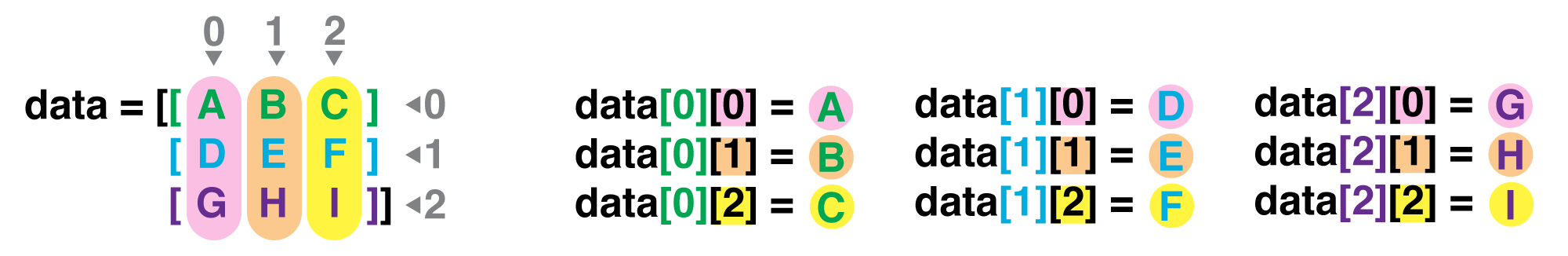
Since our array X has multiple axes, we need multiple indices to access particular values. We can index the nested arrays through multiple square brackets, or through a numpy-specific syntax.

print(X[0][0])  # Python syntax
print(X[0, 0])  # Numpy-specific syntax

This access scheme is depicted below.

sw-carpentry array figure

As with python lists, we can select subsets of numpy arrays through slicing.

print(X[0, :])  # Selects first row
print(X[:, 0])  # Selects first column

The : operator returns all entries in along the selected axis.

Unlike base python lists, numpy provides additional indexing facilities. For instance, we can perform logical indexing.

ind_threshold = np.min(X, axis=0) > 1
print(ind_threshold)  # A set of boolean values
X[:, ind_threshold]  # Logical indexing

Combining these features allows us to carry out complex data operations using syntax less like programming and more like mathematical notation.

Q8: Array operations¶

Repeat Q7 above using numpy arrays. Use the function np.sum() with the axis keyword argument, and use conditionals to create an array of indices corresponding to the valid compositions.

###
# TASK: Filter the compositions below
# TODO: Use numpy arrays and functions to repeat Q7
# The numpy function np.sum(array, axis=i) will
# take the sum over the i-th axis
###
Y = np.array(composition_fractions)
# -- WRITE YOUR CODE BELOW ----

# -- PRINT THE ANSWER -----
Y_valid

Additional Features¶

Getting help¶

If there is a python function that is mysterious to you, you can always consult the documentation. You can call the python built-in help() function on an object to display its documentation. The following documentation for list points to a number of functions that operate on lists that we did not cover; for instance, the list.sort() method is extremely useful for data science.

help(list)

There is a caveat here, which is that help() will generally provide very technical details on the object in question, which is useful for reference, but often unhelpful when first learning. If you find a particular python object very mysterious, try to formulate your question and type it into Google. Learning how to find useful information about programming concepts is one of the key skills of learning to program well.

Jupyter help shortcut

Note that in Jupyter, there’s another way to access documentation on a function. If you move your cursor over a function, click there, and press Shift + Tab, this will open a documentation panel for easy reference!

Save, close, quit, and re-open this notebook¶

You can save by clicking the floppy-disk icon in the top-left of this notebook pane, and can close the notebook by clicking the “X” of its tab. Re-open by double-clicking on 01_python_assignment.ipynb in the left-hand navigation pane.

You should find that everything is exactly as you had left it! You will have to re-run the cells to load variables, but having the output saved can be helpful.

Survey¶

Once you complete this activity, please fill out the following 30-second survey:

Survey link

Additional notebook tips¶

Save your notebooks frequently! Use the “Save” icon at the top or the Ctrl+S/Cmd+S shortcut.
Use Shift+Enter to run a cell and move on to the next cell. This allows you to sequentially execute all the cells in your notebook.
Restart & Clear Output. This option is found under the Kernel menu. It is extremely helpful to reset all code cell executions, stale package imports, and variable values.
Take the time to explore other menu options and tinker around. There’s a ton of keyboard shortcuts and nifty customizations you can do with notebooks.

Jupyter magic functions¶

Magic functions are a set of commands exclusively for Jupyter notebooks that are part of what makes notebooks so powerful. All magic commands start with a % sign, and we give examples of some below.

import numpy as np

# This command will output how long it takes the following inline command to run
%time np.mean(np.random.randint(low=1, high=7, size=1000))

# You'll see this command later; it allows Jupyter to render plots
# as output in the notebook instead of opening a new window.
%matplotlib inline

# This shows which variables are in your environment.
# Can be packages, functions, variables, and more!
%who

# You'll see this command later; it allows Jupyter to automatically
# pick up on changes in referenced code without reloading the kernel.
%load_ext autoreload

# This command will list your system environment variables.
%env

Data Extraction and Management

Intro to Data Wrangling and Tidy Data

Materials Informatics 101

Intro to Python and Jupyter Notebooks

Contents

Intro to Python and Jupyter Notebooks¶

Learning outcomes¶

Highest-level View¶

Python¶

Jupyter¶

How to use this Notebook¶

Q0: An example question¶

Jupyter Introduction¶

Cells¶

Q1: Create a new cell¶

Types of cells¶

Edit and format / execute cells¶

Code cells¶

Python Introduction¶

Simple operations¶

Q2: Average some values¶

Variables¶

Q3: Display a variable¶

Lists¶

Q4: Working with lists¶

Indexing and Slicing¶

Q5: Take the middle¶

Modules¶

Q6: Do the math¶

Conditionals and logic¶

Loops¶

Q7: Filter some data¶

Numpy arrays¶

Q8: Array operations¶

Additional Features¶

Getting help¶

Save, close, quit, and re-open this notebook¶

Survey¶

Additional notebook tips¶

Jupyter magic functions¶