Intro to Data Wrangling and Tidy Data
Contents
Intro to Data Wrangling and Tidy Data
Author: Zach del Rosario
Learning outcomes
By working through this notebook, you will be able to:
Understand basic principles of working with data in software
State the basic ideas of tidy data
State the basic ideas of data wrangling
Setup
In this day exercise, we’ll make use of the Pandas and Grama packages to work with data. Pandas is a package for data analysis, and it supplies the DataFrame object for representing data. Grama builds on top of Pandas to provide pipeline-based tools for data and machine learning.
This notebook focuses on introducing ideas, the evening notebook will teach you the mechanics of how to use these tools.
import numpy as np
import pandas as pd
import grama as gr
%matplotlib inline

DF = gr.Intention()

# For downloading data
import os
import requests
The following code downloads the same data you extracted in the previous day’s Tabula exercise.
# Filename for local data
filename_data = "./data/tabula-weibull.csv"

# The following code downloads the data, or (after downloaded)
# loads the data from a cached CSV on your machine
if not os.path.exists(filename_data):
    # Make request for data
    url_data = "https://raw.githubusercontent.com/zdelrosario/mi101/main/mi101/data/tabula-weibull1939-table4.csv"
    r = requests.get(url_data, allow_redirects=True)
    open(filename_data, 'wb').write(r.content)
    print("   Tabula-extracted data downloaded from public Google sheet")
else:
    # Note data already exists
    print("   Tabula-extracted data loaded locally")

# Read the data into memory
df_tabula = pd.read_csv(filename_data)
These are data on the tensile strength of specimens of stearic acid and plaster-of-paris.
df_tabula
Note that Pandas renamed some columns to avoid giving us duplicate column names. The names are useful for holding metadata, but shorter column names are far easier to work with in a computational environment.
Q1: Complete the code below to rename the columns
Hint: You can click-and-drag on the DataFrame printout above for a less error-prone way of giving the original column names.
###
# TASK: Copy the original column names into the double-quote below
#       to complete the code and rename the columns with shorter
#       names.
###

df_q1 = (
    df_tabula
    >> gr.tf_rename(
## TASK: Uncomment these lines and fill-in the new (short) column names
#         obs_1="",   # Observation Number, Block 1
#         area_1="",  # Specimen area, Block 1
#         sigma_1="", # Stress, Block 1
#         obs_2="",   # Observation Number, Block 2
#         area_2="",  # Specimen area, Block 2
#         sigma_2="", # Stress, Block 2

    )
)

## NOTE: No need to edit, this will show your renamed data
df_q1
Use the following to check your work:
## NO NEED TO EDIT; use this to check your work
assert(set(df_q1.columns) == {"obs_1", "area_1", "sigma_1", "obs_2", "area_2", "sigma_2"})
print("Success!")
Now the column names are much shorter, but they are far less interpretable. To help keep track of what each column means, we can construct a data dictionary.
Q2: Complete the data dictionary below to document the units associated with the short column names.
Note: Weibull in his (1939) paper reports these stress values in units kg / mm^2. This is strange; we’ll return to this later!
df_tabula.head()
TASK: Complete the text below. (Note: You can double-click on this cell to start editing it!)
Column |
Units |
|---|---|
|
(Unitless) |
|
??? |
|
??? |
|
??? |
|
??? |
|
??? |
Pivoting
Note that the data are in a rather strange layout; the first three columns report the specimen number (obs_1), cross-sectional area (area_1), and measured stress (sigma_1) for all the observations up to 13. Then the last three columns report the same quantities starting at observation 14. This sort of layout with “two blocks” is convenient for reporting values in a compact form, but it is highly inconvenient for doing analysis, as we’ll see next.
df_q1.head()
Imagine we wanted to compute some simple statistics on these data, say the mean of the stress values. Since the data come in two blocks, we have to access them separately:
sigma_mean_1 = df_q1.sigma_1.mean()
sigma_mean_2 = df_q1.sigma_2.mean()

print("Mean 1: {0:4.3f}".format(sigma_mean_1))
print("Mean 2: {0:4.3f}".format(sigma_mean_2))
We could do something hacky to combine the two:
sigma_mean_both = (12 * sigma_mean_1 + 11 * sigma_mean_2) / (12 + 11)
print("Mean both: {0:4.3f}".format(sigma_mean_both))
But it would be far easier if we could just combine all the relevant columns so they’re not in “blocks.” This is what pivoting a dataset allows us to do:
## NOTE: No need to edit; you'll learn this in the evening's notebook
df_long = (
    df_q1
    >> gr.tf_pivot_longer(
        columns=["obs_1", "area_1", "sigma_1", "obs_2", "area_2", "sigma_2"],
        names_to=[".value", "block"],
        names_sep="_",
    )
    >> gr.tf_arrange(DF.obs)
)
df_long
Pivoting is one of the key tools we need to tidy our data.
Tidy Data
Tidy data is a very simple—but very powerful—idea. The image below gives the definition of tidy data.
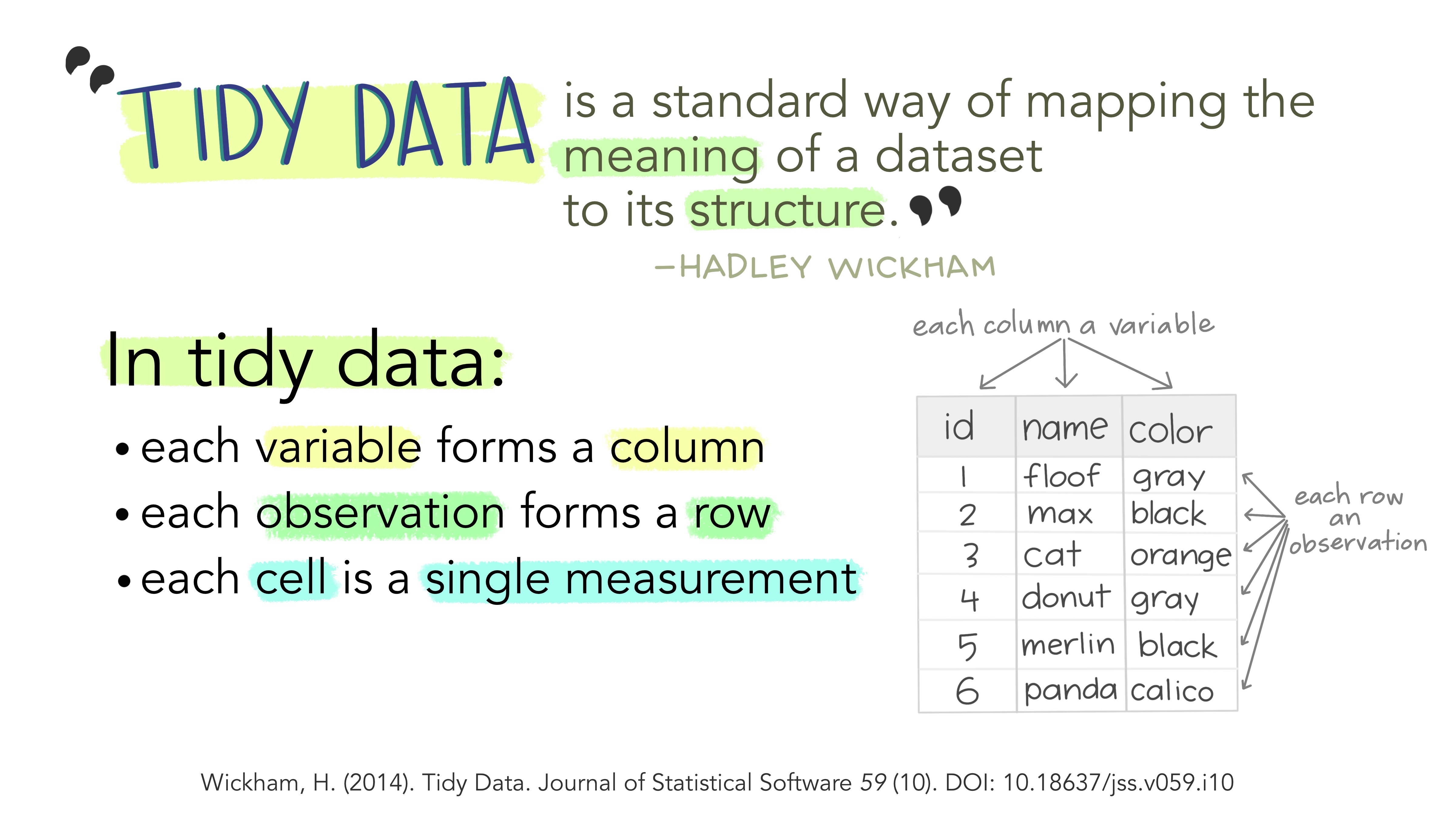
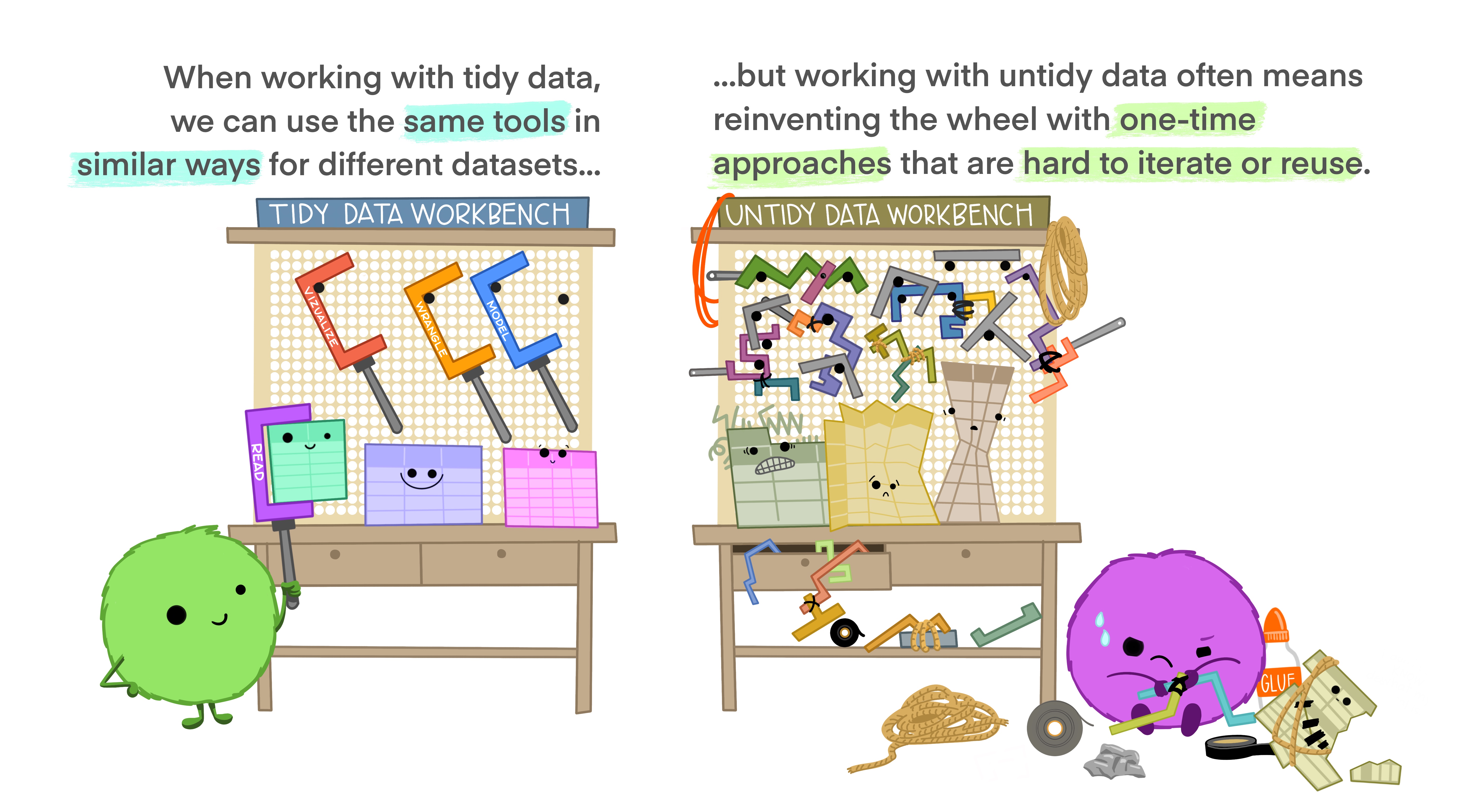
Artwork by Allison Horst, generously released under an open-source license!
The big payoff of making your data tidy is that you don’t have to build special-purpose tools to work with your data. Since every untidy dataset is untidy in its own unique (hideous) way, you would have to build special-purpose tools for every untidy dataset. By having one standard form of data, you can use the same tools for every dataset.
Let’s apply these ideas to the data we extracted using Tabula.
Q3: Inspect the original form of the data. Why are these data not tidy? How would you make the data tidy?
## NO NEED TO EDIT; run and inspect
df_tabula.head()
(Your response here)
Data Wrangling
Even once our data are tidy, they still might not be as usable as we might like. Another, less well-defined aspect of making data usable is wrangling the data into a more useful form. We’ll talk about a few aspects we might need to wrangle our data to fix: unit conversion, filtering, and data types.
Unit conversion
Weibull reports the \(\sigma_d\) values in kg / mm^2; if we interpret kg as a kilogram (mass) then these can’t be stress values! (Stress has units of force per area.) However, suppose for a moment that he were using kg to denote a kilogram-force, where \(1 \text{kgf} = 1 \text{kg} \times 9.8 m/s^2\).
Weibull gives a summary value for the same stress in the more interpretable units g / (cm s^2). Let’s check this hypothesis by comparing the proposed unit converstion with our data:
# (540 x 10^5 g/(cm s^2)) / (980 cm/s^2) * (kg / 1000 g) * (cm^2 / 100 mm^2)
print("Calculated sigma: {0:4.3f}".format(540e5 / 980 / 1000 / 100))
df_long.head()
This is very near the sigma values we have in our dataset, which lends a great deal of credibility to our interpretation of kg as kgf. With this determined, we can make a unit conversation to more standard units.
Q4: Convert the units to MPa.
Replace the factor of 1.0 below to convert the units to MPa.
###
# TASK: Replace the 1.0 factor with the correct conversion factor
###


df_q4 = (
    df_long
    >> gr.tf_mutate(sigma_MPa=DF.sigma * 1.0) # Replace 1.0 with correct factor

)

df_q4.head()
Filtering invalid values
If we take a look at the end of the dataset, we see some strange NaN entries:
## NOTE: No need to edit
df_q4.tail()
The value NaN is a special value that denotes Not a Number. Essentially, this is the way we represent something invalid. NaN can represent a missing value, a failed type conversion, or any of a variety of ways something can fail to be a number.
Often, the way we deal with NaN values is simply to remove the offending row from our dataset. We can do that with a filter operation:
## NOTE: No need to edit
df_filtered = (
    df_q4
    >> gr.tf_filter(gr.not_nan(DF.sigma_MPa))
)
df_filtered
Converting types
Lastly, it’s worth noting that all of our columns have a data type associated with them. We can inspect that type with the dtypes attribute.
## NOTE: No need to edit
df_q4.dtypes
The float64 is a way of representing a decimal value. The area and stress values we’d expect to be decimal values, but what’s up with block and obs? We’d expect those to be integers. If the types of your columns are not what you’d expect, you can do a type conversion to attempt a converstion from one data type to a desired type.
## NOTE: No need to edit
df_converted = (
    df_filtered
    >> gr.tf_mutate(
        block=gr.as_int(DF.block),
        obs=gr.as_int(DF.obs),
    )
)
df_converted.dtypes
We’ll see more about casting in the evening notebook. But now, we have a tidy and wrangled dataset!
## NOTE: No need to edit
df_converted
Bonus: The Payoff of Tidying and Wrangling
As a preview for why we want to learn how to tidy and wrangle data, let’s see what some of these tidy data tools will allow us to do. Using ggplot, we can very quickly construct simple graphs:
## NOTE: No need to edit
(
    df_converted
    >> gr.ggplot(gr.aes("area", "sigma_MPa"))
    + gr.geom_point()
)
Part of the power of plotnine (over other graphing software) is that we can very easily tweak our graphs to show additional information. For instance, if we also wanted to see if the samples in the two blocks were at all different, we could easily color the points.
## NOTE: No need to edit
(
    df_converted
    >> gr.ggplot(gr.aes("area", "sigma_MPa"))
#     + gr.geom_point() # Original
    + gr.geom_point(gr.aes(color="block")) # Modified for color
)
We’ll learn more about ggplot and visualization in tomorrow’s workshop exercises.