5. A Brief Introduction to Data Tools#

This book is about scientific modeling. However, we’ll have a much easier time working with models if we can format input data for the model and wrangle output data from the model. We will use data both to plan how to evaluate a model and to analyze the results from the model. This chapter is a brief introduction to data tools in py-grama.

Learning Objectives In this chapter, you will learn:

the fundamentals of visualizing with ggplot,
how to isolate rows with gr.tf_filter(),
how to derive values with gr.tf_mutate(),
how to derive summaries with gr.tf_group_by() and gr.tf_summarize(),
how to re-order data rows (gr.tf_arrange()) and columns (gr.tf_select()), and
how to reshape data with gr.tf_pivot_longer() and gr.tf_pivot_wider().

Note: This section assumes you have already read Chapter 4.

import grama as gr
import pandas as pd

DF = gr.Intention()
%matplotlib inline

from myst_nb import glue
gr.hide_traceback() # Shorten error traceback (for printed book)
gr.set_uqtheme()

5.1. Python Packages#

There are two python packages we’ll use to work with data:

Pandas provides the DataFrame object we’ll use to represent datasets [pandas development team, 2020].
Grama provides “verbs” to work with data [del Rosario, 2020].

As discussed in Chapter 4, transformation verbs accept a DataFrame as their input and return a DataFrame as their output. There are many useful types of transformation: We’ll illustrate these with the example dataset shown here:

# Load the data
from grama.data import df_stang
# Show the data
df_stang

	thick	alloy	E	mu	ang
0	0.022	al_24st	10600	0.321	0
1	0.022	al_24st	10600	0.323	0
2	0.032	al_24st	10400	0.329	0
3	0.032	al_24st	10300	0.319	0
4	0.064	al_24st	10500	0.323	0
...	...	...	...	...	...
71	0.064	al_24st	10400	0.327	90
72	0.064	al_24st	10500	0.320	90
73	0.081	al_24st	9900	0.314	90
74	0.081	al_24st	10000	0.316	90
75	0.081	al_24st	9900	0.314	90

76 rows × 5 columns

This is a dataset of the measured properties of several specimens made according to the same aluminum alloy specification. Due to manufacturing variability, the specimens do not have identical properties. Further details on this dataset are given in Appendix 11.1.2.

5.2. Visualizing#

One of the most powerful tools we have for making sense of data is visualization—creating plots of our data. The py-grama package uses plotnine for data visualization. A plot is created using functional programming-style code (Chapter 4.2.3), initialized with the function gr.ggplot(). The following code shows how to make a simple plot of the aluminum alloy dataset:

p = (
    # Start with a dataset
    df_stang
    ## Start the plot
    # Assign DataFrame columns to aesthetics (aes)
    >> gr.ggplot(gr.aes(x="E", y="mu", color="thick"))
    # Visualize with points
    + gr.geom_point()
)

%%capture --no-display
print(p)

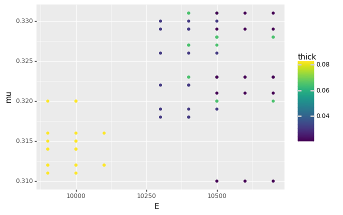
Fig. 5.1 A basic plot of the aluminum alloy dataset.#

With three lines of code, we are able to make a simple plot of the data (Figure 5.1). The philosophy behind this code is the grammar of graphics—ggplot—which is a structured way of composing elements to make a plot.

The most important concept in ggplot is the set of aesthetics, which are assigned using the gr.aes() function. We use aesthetics to map columns in a dataset to elements of the plot. To create Figure 5.1, we assigned three columns to the x-axis, y-axis, and color in the plot. Once we have chosen how to assign aesthetics, we must choose a geometry to visualize the data. We chose to use points using gr.geom_point(), which creates a scatterplot.

p = (
    df_stang
    # Start a plot object
    >> gr.ggplot(
        gr.aes(
            x="E",         # Show `E` using the x-axis
            y="mu",        # Show `mu` using the y-axis
            color="thick", # Show `thick` using color
        )
    )
    # Visualize with points
    + gr.geom_point()
)

While the code above is often quick to write, it does not produce a visually appealing graph. We can use a variety of tweaks to “beautify” the plot.

p = (
    # Start with a dataset
    df_stang
    # Convert numbers to factors (for discrete color)
    >> gr.tf_mutate(thick=gr.as_str(DF.thick))
    # Assign DataFrame columns to aesthetics (aes)
    >> gr.ggplot(gr.aes(x="E", y="mu", color="thick"))
    # Visualize with points
    + gr.geom_point(size=2)
    # Set a pleasing color scale
    + gr.scale_color_brewer(
        name="Thickness (in)", 
        type="qual",  palette=2,
    )
    # Modify the plot theme
    + gr.theme_uqbook()
    # Add more informative axis labels
    + gr.labs(
        x="Elasticity (ksi)",
        y="Poisson's Ratio (-)",
    )
)

%%capture --no-display
print(p)

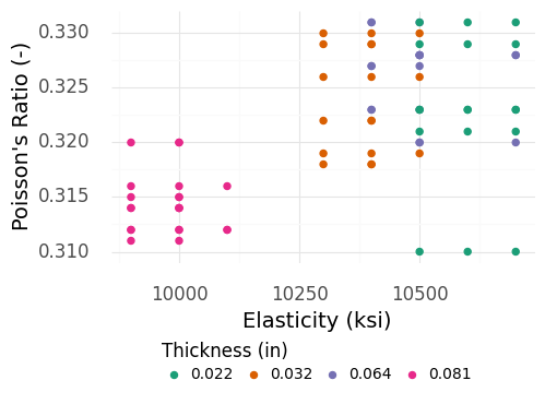
Fig. 5.2 A “beautified” plot of the aluminum alloy dataset.#

Figure 5.2 shows the “beautified” plot of the aluminum alloy data. Note that this code is much longer than the simpler version. Throughout the book, we report some—but not all—plotting code, in order to save space.

For a more thorough introduction to ggplot, consult Wickham and Grolemund [2023].

5.3. DataFrame Constructors#

In some cases, we need to quickly generate a DataFrame; for instance, to make a demo plot or to set the input values for a py-grama model. Grama provides several DataFrame constructors. The simplest constructor is gr.df_make(), which makes a DataFrame based on provided arrays.

gr.df_make(
    x=[1, 2, 3],
    c=["a", "b", "c"],
)

	x	c
0	1	a
1	2	b
2	3	c

Note that we can mix datatypes among the columns, just as with a Pandas DataFrame. However, the columns must all be of the same length or be length 1. Length 1 inputs will be recycled, as illustrated here:

# Illustrate "recycling" a single value
gr.df_make(x=[1, 2, 3], c="a")

	x	c
0	1	a
1	2	a
2	3	a

We can also use the gr.linspace() tool to help create a linearly spaced set of values. Combined with other data tools (such as gr.tf_mutate()), this allows us to quickly generate small datasets:

(
    # Create an array of 6 equispaced values
    gr.df_make(x=gr.linspace(0, 1, 6))
    # Compute y = 2x
    >> gr.tf_mutate(y=DF.x * 2)
)

	x	y
0	0.0	0.0
1	0.2	0.4
2	0.4	0.8
3	0.6	1.2
4	0.8	1.6
5	1.0	2.0

While gr.df_make() lets us construct the columns directly, it is sometimes helpful to build a grid of values. This is what gr.df_grid() does:

# Demonstrate a simple "grid" of data
gr.df_grid(
    x=[1, 2, 3],
    y=[-1, +1],
)

	x	y
0	1	-1
1	2	-1
2	3	-1
3	1	1
4	2	1
5	3	1

Note that gr.df_grid() creates a row for every combination of the inputs. For this reason, the input arrays do not need to have identical lengths.

5.4. Filtering#

The gr.tf_filter() verb helps us identify rows in a dataset that satisfy some property. For instance, the following code filters the dataset to show only those aluminum plate measurements taken at an angle of 45 degrees:

(
    df_stang
    # Keep only the rows with the specified angle
    >> gr.tf_filter(DF.ang == 45)
    # Show the first 6 rows only
    >> gr.tf_head(6)
)

	thick	alloy	E	mu	ang
0	0.022	al_24st	10700	0.321	45
1	0.022	al_24st	10500	0.323	45
2	0.032	al_24st	10400	0.329	45
3	0.032	al_24st	10500	0.319	45
4	0.064	al_24st	10400	0.323	45
5	0.064	al_24st	10500	0.328	45

We can combine multiple filters in a single statement, as in the following:

(
    df_stang
    >> gr.tf_filter(
        DF.ang == 45,     # Specified angle
        0.022 < DF.thick, # Minimum thickness
        DF.thick < 0.081, # Maximum thickness
    )
    # Show the first 6 rows only
    >> gr.tf_head(6)
)

	thick	alloy	E	mu	ang
0	0.032	al_24st	10400	0.329	45
1	0.032	al_24st	10500	0.319	45
2	0.064	al_24st	10400	0.323	45
3	0.064	al_24st	10500	0.328	45
4	0.032	al_24st	10400	0.318	45
5	0.032	al_24st	10500	0.326	45

Tip

Transformations do not edit the original data. Note above that calling gr.tf_filter() did not edit the original DataFrame df_stang. Instead, all transformation verbs return a new DataFrame. If we wanted to overwrite the data, we would need to re-assign the dataset.

Grama provides a few helper functions for use with gr.tf_filter(), listed in Table 5.1.

Table 5.1 Filter helper functions.#
Type	Functions
`NaN` detection	`gr.not_nan()`, `gr.is_nan()`
Set inclusion	`gr.var_in()`

The NaN detection tools are useful for cleaning up a dataset. The set inclusion tool gr.var_in() simplifies looking for particular cases when it’s easiest to enumerate all desired values:

(
    df_stang
    >> gr.tf_filter(
        # Keep if `thick` is in the provided set
        gr.var_in(DF.thick, [0.022, 0.081])
    )
    >> gr.tf_head(6)
)

	thick	alloy	E	mu	ang
0	0.022	al_24st	10600	0.321	0
1	0.022	al_24st	10600	0.323	0
2	0.081	al_24st	10000	0.315	0
3	0.081	al_24st	10100	0.312	0
4	0.081	al_24st	10000	0.311	0
5	0.022	al_24st	10700	0.321	45

5.5. Mutating#

The gr.tf_mutate() verb changes columns in the data and produces a new DataFrame. We can use this to derive new quantities or to overwrite the values of a column. For instance, the shear modulus is related to the elasticity \(E\) and Poisson’s ratio \(\mu\) via

\[G = \frac{E}{2(1 + \mu)}.\]

We can compute the shear modulus using the mutate tool with the elasticity E and Poisson’s ratio mu columns:

(
    df_stang
    >> gr.tf_mutate(
        # Compute the shear modulus
        G=DF.E / 2 / (1 + DF.mu), 
    )
    >> gr.tf_head(6)
)

	thick	alloy	E	mu	G
0	0.022	al_24st	10600	0.321	4012.112036
1	0.022	al_24st	10600	0.323	4006.046863
2	0.032	al_24st	10400	0.329	3912.716328
3	0.032	al_24st	10300	0.319	3904.473086
4	0.064	al_24st	10500	0.323	3968.253968
5	0.064	al_24st	10700	0.328	4028.614458

We can also overwrite old values. For instance, the elasticity is given in units of \(\text{kips}/\text{in}^2 = \text{ksi}\). We could convert the elasticity to \(\text{MPa}\) with the conversion factor \(1 \text{ksi} = 6.895 \text{MPa}\). Re-assigning an existing column will overwrite the old values with the new:

(
    df_stang
    >> gr.tf_mutate(
        E=DF.E * 6.895, # Convert from ksi to MPa
    )
    >> gr.tf_head(6)
)

	thick	alloy	E	mu
0	0.022	al_24st	73087.0	0.321
1	0.022	al_24st	73087.0	0.323
2	0.032	al_24st	71708.0	0.329
3	0.032	al_24st	71018.5	0.319
4	0.064	al_24st	72397.5	0.323
5	0.064	al_24st	73776.5	0.328

5.5.1. Mutation helpers#

There are a variety of operations and helper functions that we can use with gr.tf_mutate(). Table 5.2 lists some of the most important mutation helpers.

Table 5.2 Mutation helper functions.#
Type	Functions
Arithmetic operations	`DF.x + 1`, `DF.y - DF.x`, `DF.x * DF.y`, `DF.x / DF.y`, `DF.x ** DF.a` (Exponentiation)
Modular arithmetic	`DF.x // DF.y` (Floor division) `DF.x % DF.y` (Remainder)
Logical comparisons	`<`, `<=`, `>`, `>=`, `!=`, `==`
Logarithms	`gr.log(DF.x)`
Offsets	`gr.lead(DF.x)`, `gr.lag(DF.x)`
Rolling summaries	`gr.cumsum(DF.x)`, `gr.cumprod(DF.x)`, `gr.cummin(DF.x)`, `gr.cummax(DF.x)`, `gr.cummean(DF.x)`
Ranking	`gr.min_rank(DF.x)`, `gr.row_number(DF.x)`, `gr.dense_rank(DF.x)`, `gr.percent_rank(DF.x)`
Data conversion	`gr.as_numeric(DF.x)`, `gr.as_str(DF.x)`, `gr.as_factor(DF.x)`
Control	`gr.if_else()`, `gr.case_when()`

Many of these helpers are intuitive. Some of the more specialized helpers are described next.

5.5.2. Offsets#

Offset functions allow us to access values in adjacent rows. This can be useful for approximating derivatives.

(
    # Create a dataset of 6 linearly spaced points
    # between 0 and 1
    gr.df_make(x=gr.linspace(0, 1, 6))
    # Compute y = 3x
    >> gr.tf_mutate(y=3 * DF.x)
    # Estimate the slope of dy/dx
    >> gr.tf_mutate(
        # Approximate with a forward difference
        dy_dx_fwd=(gr.lead(DF.y) - DF.y) 
                 /(gr.lead(DF.x) - DF.x), 
        # Approximate with a backward difference
        dy_dx_rev=(DF.y - gr.lag(DF.y)) 
                 /(DF.x - gr.lag(DF.x)), 
        # Approximate with a central difference
        dy_dx_cen=(gr.lead(DF.y) - gr.lag(DF.y))   
                 /(gr.lead(DF.x) - gr.lag(DF.x)), 
    )
)

	x	y	dy_dx_fwd	dy_dx_rev	dy_dx_cen
0	0.0	0.0	3.0	NaN	NaN
1	0.2	0.6	3.0	3.0	3.0
2	0.4	1.2	3.0	3.0	3.0
3	0.6	1.8	3.0	3.0	3.0
4	0.8	2.4	3.0	3.0	3.0
5	1.0	3.0	NaN	3.0	NaN

Note that gr.lead() and gr.lag() return NaN (Not a Number) when attempting to access values “outside” the dataset.

Exercise: Re-coding NaNs.

Try using gr.if_else() with gr.is_nan() to re-code the NaN values in the dataset just given with some other numerical value, such as \(0\) or \(-1\).

5.5.3. Rolling summaries#

These functions compute a summary over all previous rows. For instance, we can take a cumulative mean to see how additional observations affect a summary. This is useful for assessing the convergence of an estimate.

(
    # Draw a random sample of 6 normally distributed
    # observations
    gr.df_make(r=gr.marg_mom("norm", mean=0, sd=1).r(6))
    >> gr.tf_mutate(
        # The sample mean will approach the true mean 
        # of 0; however, this convergence will be 
        # stochastic and slow. In practice, one should 
        # use a much larger sample, say n=10,000.
        mu=gr.cummean(DF.r),
    )
)

	r	mu
0	1.775939	1.775939
1	1.350580	1.563260
2	-0.735264	0.797085
3	0.621393	0.753162
4	1.108096	0.824149
5	0.364119	0.747477

5.5.4. Control#

Control helpers allow us to use programming constructs such as if/else and switch statements within gr.tf_mutate(). The gr.if_else() helper is useful for re-coding special values. It takes a comparison and provides one of two values: the first if the condition is met or the second if not (the else value).

(
    df_stang
    >> gr.tf_mutate(
        # Is the plate measurement aligned with the
        # rolling direction?
        alignment=gr.if_else(
            DF.ang == 0,   # Condition to check
            "aligned",     # Used if condition True
            "not aligned", # Used if condition False
        )
    )
    
    >> gr.tf_arrange(gr.desc(DF.E))
    >> gr.tf_head(6)
)

	thick	alloy	E	mu	ang	alignment
0	0.064	al_24st	10700	0.328	0	aligned
1	0.022	al_24st	10700	0.329	45	not aligned
2	0.022	al_24st	10700	0.323	90	not aligned
3	0.022	al_24st	10700	0.323	90	not aligned
4	0.064	al_24st	10700	0.328	0	aligned
5	0.022	al_24st	10700	0.331	90	not aligned

The gr.case_when() helper is a more general version of gr.if_else(). This tool will run multiple conditionals until a case is met, returning the value associated with that case.

(
    df_stang
    >> gr.tf_mutate(
        case=gr.case_when(
            # First conditional
            [
                DF.E < 10000, # The condition to check
                "low",        # The value to return
            ],    
            # If first is not met, then check next
            [DF.E < 10500, "middle"],
            # If no conditions are met, use this value
            [True,         "high"],
        )
    )
    
    >> gr.tf_head(6)
)

	thick	alloy	E	mu	case
0	0.022	al_24st	10600	0.321	high
1	0.022	al_24st	10600	0.323	high
2	0.032	al_24st	10400	0.329	middle
3	0.032	al_24st	10300	0.319	middle
4	0.064	al_24st	10500	0.323	high
5	0.064	al_24st	10700	0.328	high

When using gr.case_when(), be sure to provide a True case as the last option. This will be the “fallback” case if no other conditions are met.

5.5.5. Rounding numeric columns#

One useful trick with py-grama is the gr.tf_mutate_if() variant of the mutation verb. This function takes a conditional (that defines the if part) and a mutation helper. For all of the DataFrame columns, if the conditional is met, then the mutation is applied.

Practically, this tool is helpful for rounding all of the numeric columns in a DataFrame. The following code produces rounding to two decimal places:

(
    # Make some demonstration data
    gr.df_make(
        cat=["a", "b", "c"],
        x=[1, 2, 3],
        y=[gr.sqrt(2), gr.exp(1), gr.exp(2)],
    )
    # Round all numeric columns
    >> gr.tf_mutate_if(
        gr.is_numeric, 
        lambda x: gr.round(x, 2)
    )
)

	cat	x	y
0	a	1	1.41
1	b	2	2.72
2	c	3	7.39

5.6. Grouping and Summarizing#

Note that gr.tf_mutate() returns a new column value for each original row. In some cases, we want to summarize over multiple rows. The verb gr.tf_summarize() allows us to use summary functions over multiple rows.

(
    df_stang
    # Note that we use gr.tf_summarize() for summary
    # functions, not gr.tf_mutate() 
    >> gr.tf_summarize(
        # Compute two averages
        E_mean=gr.mean(DF.E),
        mu_mean=gr.mean(DF.mu),
    )
)

	E_mean	mu_mean
0	10344.736842	0.321461

5.6.1. Summary functions#

Grama provides a variety of summary functions. The most important ones are listed in Table 5.3.

Table 5.3 Summary functions.#
Type	Functions
Location	`gr.mean(DF.x)`, `gr.median(DF.x)`, `gr.min(DF.x)`, `gr.max(DF.x)`
Spread	`gr.sd(DF.x)`, `gr.var(DF.x)`, `gr.IQR(DF.x)`
Higher moments	`gr.skew(DF.x)`, `gr.kurt(DF.x)`
Quantile	`gr.quant(DF.x, p)`
Order	`gr.first(DF.x)`, `gr.nth(DF.x, n)`, `gr.last(DF.x)`
Counts	`gr.n_distinct(DF.x)` (Counts distinct values), `gr.n()` (Total count)
Logical	`gr.sum(DF.x == 0)` (Count cases where x == 0), `gr.pr(DF.g > 0)` (Probability helper)
Confidence interval helpers	`gr.mean_lo()`, `gr.mean_up()`, `gr.pr_lo()`, `gr.pr_up()`
Prediction interval helpers	`gr.pint_lo()`, `gr.pint_up()`

Many of these summary functions are named intuitively. The descriptive statistic tools for location, spread, and higher moments are described in Appendix 12. The interval helpers are tools for quantifying uncertainty, these are covered in Section 7.3.

Exercise: Filter with a summary.

How would you use gr.tf_filter() with a summary function to find the rows with the largest E value in the dataset?

5.6.2. Grouping#

Summaries are even more informative when grouped according to other columns. This approach allows you to compute summaries within different “categories” of rows. The verb gr.tf_group_by() adds grouping metadata to a DataFrame that gr.tf_summarize() can use.

(
    df_stang
    # Create a grouping according to the `ang` column
    >> gr.tf_group_by(DF.ang)
    # Compute summaries within each group
    >> gr.tf_summarize(
        E_mean=gr.mean(DF.E),
        mu_mean=gr.mean(DF.mu),
        # Compute number of rows in each group
        n=gr.n(), 
    )
    # Ungroup; use this if you plan to carry out other 
    # data operations
    >> gr.tf_ungroup()
)

	ang	E_mean	mu_mean	n
0	0	10369.230769	0.321231	26
1	45	10362.500000	0.321958	24
2	90	10303.846154	0.321231	26

We can also group by multiple variables; this will create a group for each unique combination of column values.

(
    df_stang
    # Group by two variables
    >> gr.tf_group_by(DF.ang, DF.thick)
    # Same summaries as before
    >> gr.tf_summarize(
        E_mean=gr.mean(DF.E),
        mu_mean=gr.mean(DF.mu),
        n=gr.n(),
    )
    >> gr.tf_ungroup()
    >> gr.tf_head(6)
)

	thick	ang	E_mean	mu_mean	n
0	0.022	0	10600.0	0.322833	6
1	0.032	0	10350.0	0.324000	6
2	0.064	0	10600.0	0.326167	6
3	0.081	0	10037.5	0.314250	8
4	0.022	45	10600.0	0.322833	6
5	0.032	45	10450.0	0.324000	6

Note that the values of n are smaller than when we grouped by ang only. This is because we have more groups, due to grouping on two columns rather than one.

Exercise: Filter with a grouped summary.

Can you figure out how to use gr.tf_group_by() and gr.tf_filter() with a summary function to find the rows with the largest E value in the dataset, per thick group?

5.6.3. Counting#

Combining grouping and counting rows gr.n() is so common that Grama provides a helper to do just that: gr.tf_count().

(
    df_stang
    >> gr.tf_count(DF.thick)
    # Equivalent to
    # >> gr.tf_group_by(DF.thick)
    # >> gr.tf_summarize(n=gr.n())
)

	thick	n
0	0.022	18
1	0.032	18
2	0.064	18
3	0.081	22

5.7. Re-ordering#

Being to be able to re-order your data, both in terms of rows and columns, can be very helpful. The gr.tf_arrange() and gr.tf_select() tools help you re-order your data.

5.7.1. Arranging#

The gr.tf_arrange() tool re-orders the rows of a dataset from smallest to largest (numerical value) or into alphabetical order, depending on the column datatype.

(
    df_stang
    # Sort from smallest to largest in `E`
    >> gr.tf_arrange(DF.E)
    >> gr.tf_head(6)
)

	thick	alloy	E	mu	ang
0	0.081	al_24st	9900	0.314	90
1	0.081	al_24st	9900	0.312	45
2	0.081	al_24st	9900	0.311	90
3	0.081	al_24st	9900	0.315	90
4	0.081	al_24st	9900	0.312	45
5	0.081	al_24st	9900	0.316	45

The gr.tf_arrange() verb also works on strings.

(
    # Make a simple example dataset
    gr.df_make(
        fruit=["blueberries", "apples", "carrots"]
    )
    # Arrange by fruit name
    >> gr.tf_arrange(DF.fruit)
)

	fruit
0	apples
1	blueberries
2	carrots

We can sort from largest to smallest by negating a variable. Because this code is a bit illegible, Grama also provides the helper gr.desc() to promote readability.

(
    df_stang
    # This would also sort large-to-small
    # >> gr.tf_arrange(-DF.E) 
    # We can use gr.desc() to reverse the sort
    >> gr.tf_arrange(gr.desc(DF.E))
    >> gr.tf_head(6)
)

	thick	alloy	E	mu	ang
0	0.064	al_24st	10700	0.328	0
1	0.022	al_24st	10700	0.329	45
2	0.022	al_24st	10700	0.323	90
3	0.022	al_24st	10700	0.323	90
4	0.064	al_24st	10700	0.328	0
5	0.022	al_24st	10700	0.331	90

The gr.desc() helper also enables reverse alphabetical sorting.

(
    gr.df_make(
        fruit=["blueberries", "apples", "carrots"]
    )
    # Reverse alphabetical sort
    >> gr.tf_arrange(gr.desc(DF.fruit))
)

	fruit
0	carrots
1	blueberries
2	apples

5.7.2. Column selection#

The gr.tf_select() helper allows us to re-order and down-select columns. This is helpful when we have a dataset that is “wide.” For instance, the Stang et al. [Stang et al., 1946] dataset is reported in the following wide format:

from grama.data import df_stang_wide
df_stang_wide.head(3)

	thick	E_00	mu_00	E_45	mu_45	E_90	mu_90	alloy
0	0.022	10600	0.321	10700	0.329	10500	0.310	al_24st
1	0.022	10600	0.323	10500	0.331	10700	0.323	al_24st
2	0.032	10400	0.329	10400	0.318	10300	0.322	al_24st

In this form of the data, the angle of the measurement is stored in the column name.

We can select a smaller number of columns to make a more focused presentation of the data. For instance, the following code selects only those columns taken at a \(0^{\circ}\) angle.

(
    df_stang_wide
    # Choose just three columns
    >> gr.tf_select(DF.thick, DF.E_00, DF.mu_00)
    >> gr.tf_head()
)

	thick	E_00	mu_00
0	0.022	10600	0.321
1	0.022	10600	0.323
2	0.032	10400	0.329
3	0.032	10300	0.319
4	0.064	10500	0.323

5.7.3. Selection helpers#

Grama also provides a number of selection helpers, which are listed in Table 5.4.

Table 5.4 Selection helper functions.#
Helper	Selects
`gr.starts_with(s)`	Columns that start with string `s`
`gr.ends_with(s)`	Columns that end with string `s`
`gr.contains(s)`	Columns that contain the string `s`
`gr.matches(s)`	Columns that match the string pattern `s`
`gr.everything()`	All columns not already selected

For instance, we can use the gr.contains() helper on the df_stang_wide to programmatically select the \(0^{\circ}\) measurements.

(
    df_stang_wide
    # Select all columns whose *name* contains "00"
    >> gr.tf_select(DF.thick, gr.contains("00"))
    >> gr.tf_head()
)

	thick	E_00	mu_00
0	0.022	10600	0.321
1	0.022	10600	0.323
2	0.032	10400	0.329
3	0.032	10300	0.319
4	0.064	10500	0.323

The gr.everything() helper may seem frivolous at first, but this is extremely helpful for re-ordering columns. Using gr.everything(), we can move a set of columns to the far left of the DataFrame without dropping any columns.

(
    df_stang_wide
    >> gr.tf_select(DF.alloy, DF.thick, gr.everything())
    >> gr.tf_head()
)

	alloy	thick	E_00	mu_00	E_45	mu_45	E_90	mu_90
0	al_24st	0.022	10600	0.321	10700	0.329	10500	0.310
1	al_24st	0.022	10600	0.323	10500	0.331	10700	0.323
2	al_24st	0.032	10400	0.329	10400	0.318	10300	0.322
3	al_24st	0.032	10300	0.319	10500	0.326	10400	0.330
4	al_24st	0.064	10500	0.323	10400	0.331	10400	0.327

5.8. Reshaping (Pivoting)#

The df_stang_wide dataset just discussed illustrates an important point about data: Datasets often come in a format that is not yet usable. Grama is built around the concept of tidy data [Wickham, 2014]: that all datasets should be formatted such that

Each variable forms a column.
Each observation forms a row.
Each type of observational unit forms a table.

The dataset we just discussed is not tidy, because one of the variables (measurement angle) is not “inside” the table but rather is misplaced in the column names. We can use a technique called pivoting to reshape df_stang_wide into a tidy dataset.

Note: What follows is a brief tour of data pivoting. For more details on pivoting, see Chapter 6 of Wickham and Grolemund [2023].

The following dataset is wide: Each column represents values measured in a single year.

# Create an example dataset with 
# multiple years of data
df_wide = pd.DataFrame({
    "1950": [1e3, 2e3],
    "1980": [2e3, 5e3],
    "2010": [4e3, 10e3],
})
df_wide

	1950	1980	2010
0	1000.0	2000.0	4000.0
1	2000.0	5000.0	10000.0

We can use gr.pivot_longer() to take a wide dataset and make it longer by transforming column names into cell values. We provide a column name for these values with names_to, and specify a new name for the previous values via values_to.

(
    df_wide
    # Start a data pivot
    >> gr.tf_pivot_longer(
        # Which columns to use? (Here: all of them)
        columns=gr.everything(),
        # What to call the new column that contains
        # the old column names
        names_to="year",
        # What to call the new column that contains
        # the old column values
        values_to="value",
    )
)

	year	value
0	1950	1000.0
1	1950	2000.0
2	1980	2000.0
3	1980	5000.0
4	2010	4000.0
5	2010	10000.0

Tidying a real dataset often requires multiple rounds of pivoting and data cleanup. For instance, using gr.tf_pivot_longer() on df_stang_wide gets us closer to a tidy dataset, but not all the way there.

(
    df_stang_wide
    # Create a unique index for each observation
    >> gr.tf_mutate(rep=DF.index)
    # Begin the data pivot
    >> gr.tf_pivot_longer(
        # Use a regular expression to match all the
        # E and mu columns, regardless of angle
        columns=gr.matches("E|mu"), 
        names_to="var",
        values_to="value",
    )
    >> gr.tf_head(6)
)

	thick	alloy	rep	var	value
0	0.022	al_24st	0	E_00	10600.0
1	0.022	al_24st	1	E_00	10600.0
2	0.032	al_24st	2	E_00	10400.0
3	0.032	al_24st	3	E_00	10300.0
4	0.064	al_24st	4	E_00	10500.0
5	0.064	al_24st	5	E_00	10700.0

Note that the variable names E and mu are concatenated with the angle values "00", "45", and "90". We can use the gr.tf_separate() tool to separate these strings using a separator character sep="_".

(
    df_stang_wide
    >> gr.tf_mutate(rep=DF.index)
    >> gr.tf_pivot_longer(
        columns=gr.matches("E|mu"),
        names_to="var",
        values_to="value",
    )
    # This will separate a column of 
    # strings into multiple columns
    >> gr.tf_separate(
        column="var",       # Which column to separate
        sep="_",            # Character for string split
        into=("name", "ang"), # New columns
    )
    >> gr.tf_head(6)
)

	thick	alloy	rep	value	name
0	0.022	al_24st	0	10600.0	E
1	0.022	al_24st	1	10600.0	E
2	0.032	al_24st	2	10400.0	E
3	0.032	al_24st	3	10300.0	E
4	0.064	al_24st	4	10500.0	E
5	0.064	al_24st	5	10700.0	E

Now we can use gr.tf_pivot_wider() to turn the variable name column values back into column headers. This completes the reshaping of the data.

(
    df_stang_wide
    >> gr.tf_mutate(rep=DF.index)
    >> gr.tf_pivot_longer(
        columns=gr.matches("E|mu"),
        names_to="var",
        values_to="value",
    )
    >> gr.tf_separate(
        column="var",
        sep="_",
        into=("name", "ang"),
    )
    # Begin another data pivot
    >> gr.tf_pivot_wider(
        # Where will the new column names come from?
        names_from="name",
        # Where will the new column values come from?
        values_from="value",
    )
    >> gr.tf_head(6)
)

	thick	alloy	rep	ang	E	mu
0	0.022	al_24st	0	00	10600.0	0.321
1	0.022	al_24st	0	45	10700.0	0.329
2	0.022	al_24st	0	90	10500.0	0.310
3	0.022	al_24st	1	00	10600.0	0.323
4	0.022	al_24st	1	45	10500.0	0.331
5	0.022	al_24st	1	90	10700.0	0.323

A more concise way to tidy the df_stang_wide dataset is to use the ".value" special keyword in gr.tf_pivot_longer(). This allows us to preserve E and mu as column names. Practically, this condenses the pivot longer and wider approach into a single verb.

(
    df_stang_wide
    # A more advanced way to pivot
    >> gr.tf_pivot_longer(
        # Match both E and mu
        columns=gr.matches("E|mu"),    
        # Use a regular expression with capture groups
        names_pattern="(E|mu)_(\\d+)", 
        # ".value" preserves E|mu as column names
        names_to=(".value", "ang"),    
    )
    >> gr.tf_head(6)
)

	thick	alloy	ang	E	mu
0	0.022	al_24st	00	10600.0	0.321
1	0.022	al_24st	45	10700.0	0.329
2	0.022	al_24st	90	10500.0	0.310
3	0.022	al_24st	00	10600.0	0.323
4	0.022	al_24st	45	10500.0	0.331
5	0.022	al_24st	90	10700.0	0.323

5.9. Further Reading#

Working with data is an important skillset. Wickham and Grolemund [2023] discuss data management in much greater detail.

All Models Are Uncertain

A Brief Introduction to Data Tools

Contents